animation/animate_decay
=====
Source
"""
=====
Decay
=====

This example showcases:

- using a generator to drive an animation,
- changing axes limits during an animation.

Output generated via `matplotlib.animation.Animation.to_jshtml`.
"""

import itertools

import matplotlib.pyplot as plt
import numpy as np

import matplotlib.animation as animation


def data_gen():
    for cnt in itertools.count():
        t = cnt / 10
        yield t, np.sin(2*np.pi*t) * np.exp(-t/10.)


def init():
    ax.set_ylim(-1.1, 1.1)
    ax.set_xlim(0, 1)
    del xdata[:]
    del ydata[:]
    line.set_data(xdata, ydata)
    return line,

fig, ax = plt.subplots()
line, = ax.plot([], [], lw=2)
ax.grid()
xdata, ydata = [], []


def run(data):
    # update the data
    t, y = data
    xdata.append(t)
    ydata.append(y)
    xmin, xmax = ax.get_xlim()

    if t >= xmax:
        ax.set_xlim(xmin, 2*xmax)
        ax.figure.canvas.draw()
    line.set_data(xdata, ydata)

    return line,

# Only save last 100 frames, but run forever
ani = animation.FuncAnimation(fig, run, data_gen, interval=100, init_func=init,
                              save_count=100)
plt.show()
animation is out of scope
animation/animated_histogram
==================
Source
"""
==================
Animated histogram
==================

Use histogram's `.BarContainer` to draw a bunch of rectangles for an animated
histogram.
"""

import functools

import matplotlib.pyplot as plt
import numpy as np

import matplotlib.animation as animation

# Setting up a random number generator with a fixed state for reproducibility.
rng = np.random.default_rng(seed=19680801)
# Fixing bin edges.
HIST_BINS = np.linspace(-4, 4, 100)

# Histogram our data with numpy.
data = rng.standard_normal(1000)
n, _ = np.histogram(data, HIST_BINS)

# %%
# To animate the histogram, we need an ``animate`` function, which generates
# a random set of numbers and updates the heights of rectangles. The ``animate``
# function updates the `.Rectangle` patches on an instance of `.BarContainer`.


def animate(frame_number, bar_container):
    # Simulate new data coming in.
    data = rng.standard_normal(1000)
    n, _ = np.histogram(data, HIST_BINS)
    for count, rect in zip(n, bar_container.patches):
        rect.set_height(count)

    return bar_container.patches

# %%
# Using :func:`~matplotlib.pyplot.hist` allows us to get an instance of
# `.BarContainer`, which is a collection of `.Rectangle` instances.  Since
# `.FuncAnimation` will only pass the frame number parameter to the animation
# function, we use `functools.partial` to fix the ``bar_container`` parameter.

# Output generated via `matplotlib.animation.Animation.to_jshtml`.

fig, ax = plt.subplots()
_, _, bar_container = ax.hist(data, HIST_BINS, lw=1,
                              ec="yellow", fc="green", alpha=0.5)
ax.set_ylim(top=55)  # set safe limit to ensure that all data is visible.

anim = functools.partial(animate, bar_container=bar_container)
ani = animation.FuncAnimation(fig, anim, 50, repeat=False, blit=True)
plt.show()

# %%
# .. tags:: plot-type: histogram, component: animation
animation is out of scope
animation/animation_demo
================
Source
"""
================
pyplot animation
================

Generating an animation by calling `~.pyplot.pause` between plotting commands.

The method shown here is only suitable for simple, low-performance use.  For
more demanding applications, look at the :mod:`.animation` module and the
examples that use it.

Note that calling `time.sleep` instead of `~.pyplot.pause` would *not* work.

Output generated via `matplotlib.animation.Animation.to_jshtml`.
"""

import matplotlib.pyplot as plt
import numpy as np

np.random.seed(19680801)
data = np.random.random((50, 50, 50))

fig, ax = plt.subplots()

for i, img in enumerate(data):
    ax.clear()
    ax.imshow(img)
    ax.set_title(f"frame {i}")
    # Note that using time.sleep does *not* work here!
    plt.pause(0.1)
animation is out of scope
animation/bayes_update
================
Source
"""
================
The Bayes update
================

This animation displays the posterior estimate updates as it is refitted when
new data arrives.
The vertical line represents the theoretical value to which the plotted
distribution should converge.

Output generated via `matplotlib.animation.Animation.to_jshtml`.
"""

import math

import matplotlib.pyplot as plt
import numpy as np

from matplotlib.animation import FuncAnimation


def beta_pdf(x, a, b):
    return (x**(a-1) * (1-x)**(b-1) * math.gamma(a + b)
            / (math.gamma(a) * math.gamma(b)))


class UpdateDist:
    def __init__(self, ax, prob=0.5):
        self.success = 0
        self.prob = prob
        self.line, = ax.plot([], [], 'k-')
        self.x = np.linspace(0, 1, 200)
        self.ax = ax

        # Set up plot parameters
        self.ax.set_xlim(0, 1)
        self.ax.set_ylim(0, 10)
        self.ax.grid(True)

        # This vertical line represents the theoretical value, to
        # which the plotted distribution should converge.
        self.ax.axvline(prob, linestyle='--', color='black')

    def start(self):
        # Used for the *init_func* parameter of FuncAnimation; this is called when
        # initializing the animation, and also after resizing the figure.
        return self.line,

    def __call__(self, i):
        # This way the plot can continuously run and we just keep
        # watching new realizations of the process
        if i == 0:
            self.success = 0
            self.line.set_data([], [])
            return self.line,

        # Choose success based on exceed a threshold with a uniform pick
        if np.random.rand() < self.prob:
            self.success += 1
        y = beta_pdf(self.x, self.success + 1, (i - self.success) + 1)
        self.line.set_data(self.x, y)
        return self.line,

# Fixing random state for reproducibility
np.random.seed(19680801)


fig, ax = plt.subplots()
ud = UpdateDist(ax, prob=0.7)
anim = FuncAnimation(fig, ud, init_func=ud.start, frames=100, interval=100, blit=True)
plt.show()

# %%
# .. tags:: component: animation, plot-type: line
animation is out of scope
animation/double_pendulum
===========================
Source
"""
===========================
The double pendulum problem
===========================

This animation illustrates the double pendulum problem.

Double pendulum formula translated from the C code at
http://www.physics.usyd.edu.au/~wheat/dpend_html/solve_dpend.c

Output generated via `matplotlib.animation.Animation.to_jshtml`.
"""

import matplotlib.pyplot as plt
import numpy as np
from numpy import cos, sin

import matplotlib.animation as animation

G = 9.8  # acceleration due to gravity, in m/s^2
L1 = 1.0  # length of pendulum 1 in m
L2 = 1.0  # length of pendulum 2 in m
L = L1 + L2  # maximal length of the combined pendulum
M1 = 1.0  # mass of pendulum 1 in kg
M2 = 1.0  # mass of pendulum 2 in kg
t_stop = 2.5  # how many seconds to simulate
history_len = 500  # how many trajectory points to display


def derivs(t, state):
    dydx = np.zeros_like(state)

    dydx[0] = state[1]

    delta = state[2] - state[0]
    den1 = (M1+M2) * L1 - M2 * L1 * cos(delta) * cos(delta)
    dydx[1] = ((M2 * L1 * state[1] * state[1] * sin(delta) * cos(delta)
                + M2 * G * sin(state[2]) * cos(delta)
                + M2 * L2 * state[3] * state[3] * sin(delta)
                - (M1+M2) * G * sin(state[0]))
               / den1)

    dydx[2] = state[3]

    den2 = (L2/L1) * den1
    dydx[3] = ((- M2 * L2 * state[3] * state[3] * sin(delta) * cos(delta)
                + (M1+M2) * G * sin(state[0]) * cos(delta)
                - (M1+M2) * L1 * state[1] * state[1] * sin(delta)
                - (M1+M2) * G * sin(state[2]))
               / den2)

    return dydx

# create a time array from 0..t_stop sampled at 0.01 second steps
dt = 0.01
t = np.arange(0, t_stop, dt)

# th1 and th2 are the initial angles (degrees)
# w10 and w20 are the initial angular velocities (degrees per second)
th1 = 120.0
w1 = 0.0
th2 = -10.0
w2 = 0.0

# initial state
state = np.radians([th1, w1, th2, w2])

# integrate the ODE using Euler's method
y = np.empty((len(t), 4))
y[0] = state
for i in range(1, len(t)):
    y[i] = y[i - 1] + derivs(t[i - 1], y[i - 1]) * dt

# A more accurate estimate could be obtained e.g. using scipy:
#
#   y = scipy.integrate.solve_ivp(derivs, t[[0, -1]], state, t_eval=t).y.T

x1 = L1*sin(y[:, 0])
y1 = -L1*cos(y[:, 0])

x2 = L2*sin(y[:, 2]) + x1
y2 = -L2*cos(y[:, 2]) + y1

fig = plt.figure(figsize=(5, 4))
ax = fig.add_subplot(autoscale_on=False, xlim=(-L, L), ylim=(-L, 1.))
ax.set_aspect('equal')
ax.grid()

line, = ax.plot([], [], 'o-', lw=2)
trace, = ax.plot([], [], '.-', lw=1, ms=2)
time_template = 'time = %.1fs'
time_text = ax.text(0.05, 0.9, '', transform=ax.transAxes)


def animate(i):
    thisx = [0, x1[i], x2[i]]
    thisy = [0, y1[i], y2[i]]

    history_x = x2[:i]
    history_y = y2[:i]

    line.set_data(thisx, thisy)
    trace.set_data(history_x, history_y)
    time_text.set_text(time_template % (i*dt))
    return line, trace, time_text


ani = animation.FuncAnimation(
    fig, animate, len(y), interval=dt*1000, blit=True)
plt.show()
animation is out of scope
animation/dynamic_image
=================================================
Source
"""
=================================================
Animated image using a precomputed list of images
=================================================

Output generated via `matplotlib.animation.Animation.to_jshtml`.
"""

import matplotlib.pyplot as plt
import numpy as np

import matplotlib.animation as animation

fig, ax = plt.subplots()


def f(x, y):
    return np.sin(x) + np.cos(y)

x = np.linspace(0, 2 * np.pi, 120)
y = np.linspace(0, 2 * np.pi, 100).reshape(-1, 1)

# ims is a list of lists, each row is a list of artists to draw in the
# current frame; here we are just animating one artist, the image, in
# each frame
ims = []
for i in range(60):
    x += np.pi / 15
    y += np.pi / 30
    im = ax.imshow(f(x, y), animated=True)
    if i == 0:
        ax.imshow(f(x, y))  # show an initial one first
    ims.append([im])

ani = animation.ArtistAnimation(fig, ims, interval=50, blit=True,
                                repeat_delay=1000)

# To save the animation, use e.g.
#
# ani.save("movie.mp4")
#
# or
#
# writer = animation.FFMpegWriter(
#     fps=15, metadata=dict(artist='Me'), bitrate=1800)
# ani.save("movie.mp4", writer=writer)

plt.show()

# %%
# .. tags:: component: animation
animation is out of scope
animation/frame_grabbing_sgskip
==============
Source
"""
==============
Frame grabbing
==============

Use a MovieWriter directly to grab individual frames and write them to a
file.  This avoids any event loop integration, and thus works even with the Agg
backend.  This is not recommended for use in an interactive setting.
"""

import numpy as np

import matplotlib

matplotlib.use("Agg")
import matplotlib.pyplot as plt

from matplotlib.animation import FFMpegWriter

# Fixing random state for reproducibility
np.random.seed(19680801)


metadata = dict(title='Movie Test', artist='Matplotlib',
                comment='Movie support!')
writer = FFMpegWriter(fps=15, metadata=metadata)

fig = plt.figure()
l, = plt.plot([], [], 'k-o')

plt.xlim(-5, 5)
plt.ylim(-5, 5)

x0, y0 = 0, 0

with writer.saving(fig, "writer_test.mp4", 100):
    for i in range(100):
        x0 += 0.1 * np.random.randn()
        y0 += 0.1 * np.random.randn()
        l.set_data([x0], [y0])
        writer.grab_frame()
animation is out of scope
animation/multiple_axes
=======================
Source
"""
=======================
Multiple Axes animation
=======================

This example showcases:

- how animation across multiple subplots works,
- using a figure artist in the animation.

Output generated via `matplotlib.animation.Animation.to_jshtml`.
"""

import matplotlib.pyplot as plt
import numpy as np

import matplotlib.animation as animation
from matplotlib.patches import ConnectionPatch

fig, (axl, axr) = plt.subplots(
    ncols=2,
    sharey=True,
    figsize=(6, 2),
    gridspec_kw=dict(width_ratios=[1, 3], wspace=0),
)
axl.set_aspect(1)
axr.set_box_aspect(1 / 3)
axr.yaxis.set_visible(False)
axr.xaxis.set_ticks([0, np.pi, 2 * np.pi], ["0", r"$\pi$", r"$2\pi$"])

# draw circle with initial point in left Axes
x = np.linspace(0, 2 * np.pi, 50)
axl.plot(np.cos(x), np.sin(x), "k", lw=0.3)
point, = axl.plot(0, 0, "o")

# draw full curve to set view limits in right Axes
sine, = axr.plot(x, np.sin(x))

# draw connecting line between both graphs
con = ConnectionPatch(
    (1, 0),
    (0, 0),
    "data",
    "data",
    axesA=axl,
    axesB=axr,
    color="C0",
    ls="dotted",
)
fig.add_artist(con)


def animate(i):
    x = np.linspace(0, i, int(i * 25 / np.pi))
    sine.set_data(x, np.sin(x))
    x, y = np.cos(i), np.sin(i)
    point.set_data([x], [y])
    con.xy1 = x, y
    con.xy2 = i, y
    return point, sine, con


ani = animation.FuncAnimation(
    fig,
    animate,
    interval=50,
    blit=False,  # blitting can't be used with Figure artists
    frames=x,
    repeat_delay=100,
)

plt.show()

# %%
#
# .. admonition:: References
#
#    The use of the following functions, methods, classes and modules is shown
#    in this example:
#
#    - `matplotlib.patches.ConnectionPatch`
#    - `matplotlib.animation.FuncAnimation`
#
# .. tags:: component: axes, component: animation
animation is out of scope
animation/pause_resume
=============================
Source
"""
=============================
Pause and resume an animation
=============================

This example showcases:

- using the Animation.pause() method to pause an animation.
- using the Animation.resume() method to resume an animation.

.. note::
    This example exercises the interactive capabilities of Matplotlib, and this
    will not appear in the static documentation. Please run this code on your
    machine to see the interactivity.

    You can copy and paste individual parts, or download the entire example
    using the link at the bottom of the page.

Output generated via `matplotlib.animation.Animation.to_jshtml`.
"""

import matplotlib.pyplot as plt
import numpy as np

import matplotlib.animation as animation


class PauseAnimation:
    def __init__(self):
        fig, ax = plt.subplots()
        ax.set_title('Click to pause/resume the animation')
        x = np.linspace(-0.1, 0.1, 1000)

        # Start with a normal distribution
        self.n0 = (1.0 / ((4 * np.pi * 2e-4 * 0.1) ** 0.5)
                   * np.exp(-x ** 2 / (4 * 2e-4 * 0.1)))
        self.p, = ax.plot(x, self.n0)

        self.animation = animation.FuncAnimation(
            fig, self.update, frames=200, interval=50, blit=True)
        self.paused = False

        fig.canvas.mpl_connect('button_press_event', self.toggle_pause)

    def toggle_pause(self, *args, **kwargs):
        if self.paused:
            self.animation.resume()
        else:
            self.animation.pause()
        self.paused = not self.paused

    def update(self, i):
        self.n0 += i / 100 % 5
        self.p.set_ydata(self.n0 % 20)
        return (self.p,)


pa = PauseAnimation()
plt.show()
animation is out of scope
animation/rain
===============
Source
"""
===============
Rain simulation
===============

Simulates rain drops on a surface by animating the scale and opacity
of 50 scatter points.

Author: Nicolas P. Rougier

Output generated via `matplotlib.animation.Animation.to_jshtml`.
"""

import matplotlib.pyplot as plt
import numpy as np

from matplotlib.animation import FuncAnimation

# Fixing random state for reproducibility
np.random.seed(19680801)


# Create new Figure and an Axes which fills it.
fig = plt.figure(figsize=(7, 7))
ax = fig.add_axes((0, 0, 1, 1), frameon=False)
ax.set_xlim(0, 1), ax.set_xticks([])
ax.set_ylim(0, 1), ax.set_yticks([])

# Create rain data
n_drops = 50
rain_drops = np.zeros(n_drops, dtype=[('position', float, (2,)),
                                      ('size',     float),
                                      ('growth',   float),
                                      ('color',    float, (4,))])

# Initialize the raindrops in random positions and with
# random growth rates.
rain_drops['position'] = np.random.uniform(0, 1, (n_drops, 2))
rain_drops['growth'] = np.random.uniform(50, 200, n_drops)

# Construct the scatter which we will update during animation
# as the raindrops develop.
scat = ax.scatter(rain_drops['position'][:, 0], rain_drops['position'][:, 1],
                  s=rain_drops['size'], lw=0.5, edgecolors=rain_drops['color'],
                  facecolors='none')


def update(frame_number):
    # Get an index which we can use to re-spawn the oldest raindrop.
    current_index = frame_number % n_drops

    # Make all colors more transparent as time progresses.
    rain_drops['color'][:, 3] -= 1.0/len(rain_drops)
    rain_drops['color'][:, 3] = np.clip(rain_drops['color'][:, 3], 0, 1)

    # Make all circles bigger.
    rain_drops['size'] += rain_drops['growth']

    # Pick a new position for oldest rain drop, resetting its size,
    # color and growth factor.
    rain_drops['position'][current_index] = np.random.uniform(0, 1, 2)
    rain_drops['size'][current_index] = 5
    rain_drops['color'][current_index] = (0, 0, 0, 1)
    rain_drops['growth'][current_index] = np.random.uniform(50, 200)

    # Update the scatter collection, with the new colors, sizes and positions.
    scat.set_edgecolors(rain_drops['color'])
    scat.set_sizes(rain_drops['size'])
    scat.set_offsets(rain_drops['position'])
    return [scat]


# Construct the animation, using the update function as the animation director.
animation = FuncAnimation(fig, update, interval=10, save_count=100, blit=True)
plt.show()

# %%
# .. tags::
#
#    component: animation
#    plot-type: scatter
#    purpose: fun
animation is out of scope
animation/random_walk
=======================
Source
"""
=======================
Animated 3D random walk
=======================

Output generated via `matplotlib.animation.Animation.to_jshtml`.
"""

import matplotlib.pyplot as plt
import numpy as np

import matplotlib.animation as animation

# Fixing random state for reproducibility
np.random.seed(19680801)


def random_walk(num_steps, max_step=0.05):
    """Return a 3D random walk as (num_steps, 3) array."""
    start_pos = np.random.random(3)
    steps = np.random.uniform(-max_step, max_step, size=(num_steps, 3))
    walk = start_pos + np.cumsum(steps, axis=0)
    return walk


def update_lines(num, walks, lines):
    for line, walk in zip(lines, walks):
        line.set_data_3d(walk[:num, :].T)
    return lines


# Data: 40 random walks as (num_steps, 3) arrays
num_steps = 30
walks = [random_walk(num_steps) for index in range(40)]

# Attaching 3D axis to the figure
fig = plt.figure()
ax = fig.add_subplot(projection="3d")

# Create lines initially without data
lines = [ax.plot([], [], [])[0] for _ in walks]

# Setting the Axes properties
ax.set(xlim3d=(0, 1), xlabel='X')
ax.set(ylim3d=(0, 1), ylabel='Y')
ax.set(zlim3d=(0, 1), zlabel='Z')

# Creating the Animation object
ani = animation.FuncAnimation(
    fig, update_lines, num_steps, fargs=(walks, lines), interval=100)

plt.show()

# %%
# .. tags:: component: animation, plot-type: 3D
animation is out of scope
animation/simple_anim
========================
Source
"""
========================
Basic animated line plot
========================

Output generated via `matplotlib.animation.Animation.to_jshtml`.
"""

import matplotlib.pyplot as plt
import numpy as np

import matplotlib.animation as animation

fig, ax = plt.subplots()

x = np.arange(0, 2*np.pi, 0.01)
line, = ax.plot(x, np.sin(x))


def animate(i):
    line.set_ydata(np.sin(x + i / 50))  # update the data.
    return line,


ani = animation.FuncAnimation(
    fig, animate, interval=20, blit=True, save_count=50)

# To save the animation, use e.g.
#
# ani.save("movie.mp4")
#
# or
#
# writer = animation.FFMpegWriter(
#     fps=15, metadata=dict(artist='Me'), bitrate=1800)
# ani.save("movie.mp4", writer=writer)

plt.show()

# %%
#
# .. tags::
#    component: animation,
#    level: beginner
animation is out of scope
animation/simple_scatter
=============================
Source
"""
=============================
Animated scatter saved as GIF
=============================

Output generated via `matplotlib.animation.Animation.to_jshtml`.
"""
import matplotlib.pyplot as plt
import numpy as np

import matplotlib.animation as animation

fig, ax = plt.subplots()
ax.set_xlim(0, 10)

scat = ax.scatter(1, 0)
x = np.linspace(0, 10)


def animate(i):
    scat.set_offsets((x[i], 0))
    return (scat,)


ani = animation.FuncAnimation(fig, animate, repeat=True, frames=len(x) - 1, interval=50)

# To save the animation using Pillow as a gif
# writer = animation.PillowWriter(fps=15,
#                                 metadata=dict(artist='Me'),
#                                 bitrate=1800)
# ani.save('scatter.gif', writer=writer)

plt.show()

# %%
#
# .. tags::
#    component: animation,
#    plot-type: scatter,
#    purpose: reference,
#    level: intermediate
animation is out of scope
animation/strip_chart
============
Source
"""
============
Oscilloscope
============

Emulates an oscilloscope.

Output generated via `matplotlib.animation.Animation.to_jshtml`.
"""

import matplotlib.pyplot as plt
import numpy as np

import matplotlib.animation as animation
from matplotlib.lines import Line2D


class Scope:
    def __init__(self, ax, maxt=2, dt=0.02):
        self.ax = ax
        self.dt = dt
        self.maxt = maxt
        self.tdata = [0]
        self.ydata = [0]
        self.line = Line2D(self.tdata, self.ydata)
        self.ax.add_line(self.line)
        self.ax.set_ylim(-.1, 1.1)
        self.ax.set_xlim(0, self.maxt)

    def update(self, y):
        lastt = self.tdata[-1]
        if lastt >= self.tdata[0] + self.maxt:  # reset the arrays
            self.tdata = [self.tdata[-1]]
            self.ydata = [self.ydata[-1]]
            self.ax.set_xlim(self.tdata[0], self.tdata[0] + self.maxt)
            self.ax.figure.canvas.draw()

        # This slightly more complex calculation avoids floating-point issues
        # from just repeatedly adding `self.dt` to the previous value.
        t = self.tdata[0] + len(self.tdata) * self.dt

        self.tdata.append(t)
        self.ydata.append(y)
        self.line.set_data(self.tdata, self.ydata)
        return self.line,


def emitter(p=0.1):
    """Return a random value in [0, 1) with probability p, else 0."""
    while True:
        v = np.random.rand()
        if v > p:
            yield 0.
        else:
            yield np.random.rand()


# Fixing random state for reproducibility
np.random.seed(19680801 // 10)


fig, ax = plt.subplots()
scope = Scope(ax)

# pass a generator in "emitter" to produce data for the update func
ani = animation.FuncAnimation(fig, scope.update, emitter, interval=50,
                              blit=True, save_count=100)

plt.show()

# ..tags:: animation, plot-type: line
animation is out of scope
animation/unchained
====================
Source
"""
====================
Matplotlib unchained
====================

Comparative path demonstration of frequency from a fake signal of a pulsar
(mostly known because of the cover for Joy Division's Unknown Pleasures).

Author: Nicolas P. Rougier

Output generated via `matplotlib.animation.Animation.to_jshtml`.
"""

import matplotlib.pyplot as plt
import numpy as np

import matplotlib.animation as animation

# Fixing random state for reproducibility
np.random.seed(19680801)


# Create new Figure with black background
fig = plt.figure(figsize=(8, 8), facecolor='black')

# Add a subplot with no frame
ax = plt.subplot(frameon=False)

# Generate random data
data = np.random.uniform(0, 1, (64, 75))
X = np.linspace(-1, 1, data.shape[-1])
G = 1.5 * np.exp(-4 * X ** 2)

# Generate line plots
lines = []
for i in range(len(data)):
    # Small reduction of the X extents to get a cheap perspective effect
    xscale = 1 - i / 200.
    # Same for linewidth (thicker strokes on bottom)
    lw = 1.5 - i / 100.0
    line, = ax.plot(xscale * X, i + G * data[i], color="w", lw=lw)
    lines.append(line)

# Set y limit (or first line is cropped because of thickness)
ax.set_ylim(-1, 70)

# No ticks
ax.set_xticks([])
ax.set_yticks([])

# 2 part titles to get different font weights
ax.text(0.5, 1.0, "MATPLOTLIB ", transform=ax.transAxes,
        ha="right", va="bottom", color="w",
        family="sans-serif", fontweight="light", fontsize=16)
ax.text(0.5, 1.0, "UNCHAINED", transform=ax.transAxes,
        ha="left", va="bottom", color="w",
        family="sans-serif", fontweight="bold", fontsize=16)


def update(*args):
    # Shift all data to the right
    data[:, 1:] = data[:, :-1]

    # Fill-in new values
    data[:, 0] = np.random.uniform(0, 1, len(data))

    # Update data
    for i in range(len(data)):
        lines[i].set_ydata(i + G * data[i])

    # Return modified artists
    return lines

# Construct the animation, using the update function as the animation director.
anim = animation.FuncAnimation(fig, update, interval=10, save_count=100)
plt.show()

# %%
# .. tags::
#
#    component: animation
#    plot-type: line
#    purpose: fun
animation is out of scope
axes_grid1/demo_anchored_direction_arrows
========================
Source
"""
========================
Anchored Direction Arrow
========================

"""
import matplotlib.pyplot as plt
import numpy as np

import matplotlib.font_manager as fm
from mpl_toolkits.axes_grid1.anchored_artists import AnchoredDirectionArrows

# Fixing random state for reproducibility
np.random.seed(19680801)

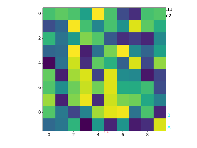
fig, ax = plt.subplots()
ax.imshow(np.random.random((10, 10)))

# Simple example
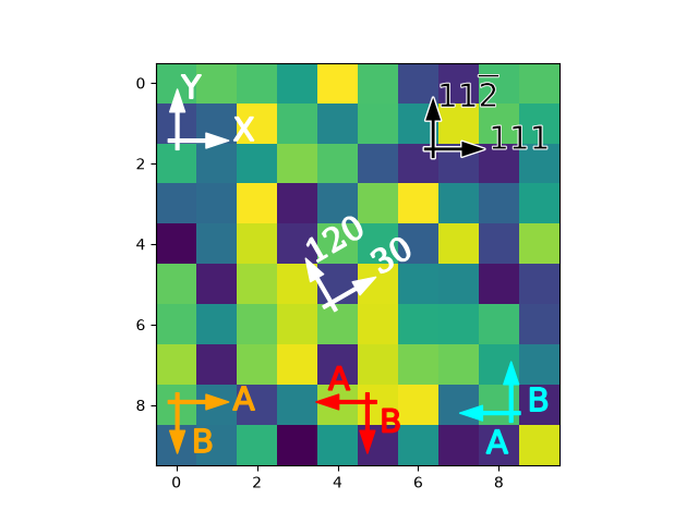
simple_arrow = AnchoredDirectionArrows(ax.transAxes, 'X', 'Y')
ax.add_artist(simple_arrow)

# High contrast arrow
high_contrast_part_1 = AnchoredDirectionArrows(
                            ax.transAxes,
                            '111', r'11$\overline{2}$',
                            loc='upper right',
                            arrow_props={'ec': 'w', 'fc': 'none', 'alpha': 1,
                                         'lw': 2}
                            )
ax.add_artist(high_contrast_part_1)

high_contrast_part_2 = AnchoredDirectionArrows(
                            ax.transAxes,
                            '111', r'11$\overline{2}$',
                            loc='upper right',
                            arrow_props={'ec': 'none', 'fc': 'k'},
                            text_props={'ec': 'w', 'fc': 'k', 'lw': 0.4}
                            )
ax.add_artist(high_contrast_part_2)

# Rotated arrow
fontprops = fm.FontProperties(family='serif')

rotated_arrow = AnchoredDirectionArrows(
                    ax.transAxes,
                    '30', '120',
                    loc='center',
                    color='w',
                    angle=30,
                    fontproperties=fontprops
                    )
ax.add_artist(rotated_arrow)

# Altering arrow directions
a1 = AnchoredDirectionArrows(
        ax.transAxes, 'A', 'B', loc='lower center',
        length=-0.15,
        sep_x=0.03, sep_y=0.03,
        color='r'
    )
ax.add_artist(a1)

a2 = AnchoredDirectionArrows(
        ax.transAxes, 'A', ' B', loc='lower left',
        aspect_ratio=-1,
        sep_x=0.01, sep_y=-0.02,
        color='orange'
        )
ax.add_artist(a2)


a3 = AnchoredDirectionArrows(
        ax.transAxes, ' A', 'B', loc='lower right',
        length=-0.15,
        aspect_ratio=-1,
        sep_y=-0.1, sep_x=0.04,
        color='cyan'
        )
ax.add_artist(a3)

plt.show()
axes_grid1/demo_axes_divider
============
Source
"""
============
Axes divider
============

Axes divider to calculate location of Axes and
create a divider for them using existing Axes instances.
"""

import matplotlib.pyplot as plt

from matplotlib import cbook


def get_demo_image():
    z = cbook.get_sample_data("axes_grid/bivariate_normal.npy")  # 15x15 array
    return z, (-3, 4, -4, 3)


def demo_simple_image(ax):
    Z, extent = get_demo_image()

    im = ax.imshow(Z, extent=extent)
    cb = plt.colorbar(im)
    cb.ax.yaxis.set_tick_params(labelright=False)


def demo_locatable_axes_hard(fig):
    from mpl_toolkits.axes_grid1 import Size, SubplotDivider

    divider = SubplotDivider(fig, 2, 2, 2, aspect=True)

    # Axes for image
    ax = fig.add_subplot(axes_locator=divider.new_locator(nx=0, ny=0))
    # Axes for colorbar
    ax_cb = fig.add_subplot(axes_locator=divider.new_locator(nx=2, ny=0))

    divider.set_horizontal([
        Size.AxesX(ax),  # main Axes
        Size.Fixed(0.05),  # padding, 0.1 inch
        Size.Fixed(0.2),  # colorbar, 0.3 inch
    ])
    divider.set_vertical([Size.AxesY(ax)])

    Z, extent = get_demo_image()

    im = ax.imshow(Z, extent=extent)
    plt.colorbar(im, cax=ax_cb)
    ax_cb.yaxis.set_tick_params(labelright=False)


def demo_locatable_axes_easy(ax):
    from mpl_toolkits.axes_grid1 import make_axes_locatable

    divider = make_axes_locatable(ax)

    ax_cb = divider.append_axes("right", size="5%", pad=0.05)
    fig = ax.get_figure()
    fig.add_axes(ax_cb)

    Z, extent = get_demo_image()
    im = ax.imshow(Z, extent=extent)

    plt.colorbar(im, cax=ax_cb)
    ax_cb.yaxis.tick_right()
    ax_cb.yaxis.set_tick_params(labelright=False)


def demo_images_side_by_side(ax):
    from mpl_toolkits.axes_grid1 import make_axes_locatable

    divider = make_axes_locatable(ax)

    Z, extent = get_demo_image()
    ax2 = divider.append_axes("right", size="100%", pad=0.05)
    fig1 = ax.get_figure()
    fig1.add_axes(ax2)

    ax.imshow(Z, extent=extent)
    ax2.imshow(Z, extent=extent)
    ax2.yaxis.set_tick_params(labelleft=False)


def demo():
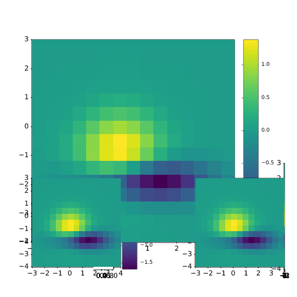
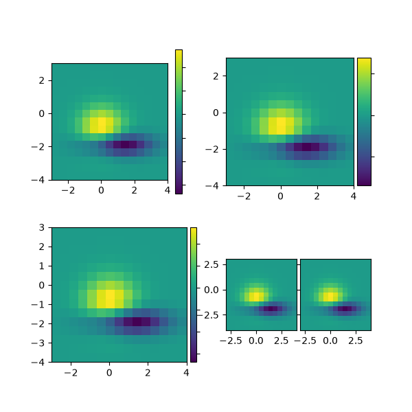
    fig = plt.figure(figsize=(6, 6))

    # PLOT 1
    # simple image & colorbar
    ax = fig.add_subplot(2, 2, 1)
    demo_simple_image(ax)

    # PLOT 2
    # image and colorbar with draw-time positioning -- a hard way
    demo_locatable_axes_hard(fig)

    # PLOT 3
    # image and colorbar with draw-time positioning -- an easy way
    ax = fig.add_subplot(2, 2, 3)
    demo_locatable_axes_easy(ax)

    # PLOT 4
    # two images side by side with fixed padding.
    ax = fig.add_subplot(2, 2, 4)
    demo_images_side_by_side(ax)

    plt.show()


demo()
axes_grid1/demo_axes_grid
==============
Source
"""
==============
Demo Axes Grid
==============

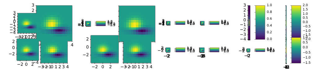
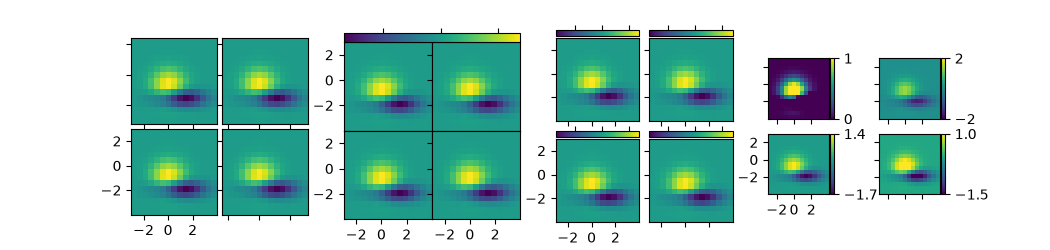
Grid of 2x2 images with a single colorbar or with one colorbar per Axes.
"""

import matplotlib.pyplot as plt

from matplotlib import cbook
from mpl_toolkits.axes_grid1 import ImageGrid

fig = plt.figure(figsize=(10.5, 2.5))
Z = cbook.get_sample_data("axes_grid/bivariate_normal.npy")  # 15x15 array
extent = (-3, 4, -4, 3)


# A grid of 2x2 images with 0.05 inch pad between images and only the
# lower-left Axes is labeled.
grid = ImageGrid(
    fig, 141,  # similar to fig.add_subplot(141).
     nrows_ncols=(2, 2), axes_pad=0.05, label_mode="1")
for ax in grid:
    ax.imshow(Z, extent=extent)
# This only affects Axes in first column and second row as share_all=False.
grid.axes_llc.set(xticks=[-2, 0, 2], yticks=[-2, 0, 2])


# A grid of 2x2 images with a single colorbar.
grid = ImageGrid(
    fig, 142,  # similar to fig.add_subplot(142).
    nrows_ncols=(2, 2), axes_pad=0.0, label_mode="L", share_all=True,
    cbar_location="top", cbar_mode="single")
for ax in grid:
    im = ax.imshow(Z, extent=extent)
grid.cbar_axes[0].colorbar(im)
for cax in grid.cbar_axes:
    cax.tick_params(labeltop=False)
# This affects all Axes as share_all = True.
grid.axes_llc.set(xticks=[-2, 0, 2], yticks=[-2, 0, 2])


# A grid of 2x2 images. Each image has its own colorbar.
grid = ImageGrid(
    fig, 143,  # similar to fig.add_subplot(143).
    nrows_ncols=(2, 2), axes_pad=0.1, label_mode="1", share_all=True,
    cbar_location="top", cbar_mode="each", cbar_size="7%", cbar_pad="2%")
for ax, cax in zip(grid, grid.cbar_axes):
    im = ax.imshow(Z, extent=extent)
    cax.colorbar(im)
    cax.tick_params(labeltop=False)
# This affects all Axes as share_all = True.
grid.axes_llc.set(xticks=[-2, 0, 2], yticks=[-2, 0, 2])


# A grid of 2x2 images. Each image has its own colorbar.
grid = ImageGrid(
    fig, 144,  # similar to fig.add_subplot(144).
    nrows_ncols=(2, 2), axes_pad=(0.45, 0.15), label_mode="1", share_all=True,
    cbar_location="right", cbar_mode="each", cbar_size="7%", cbar_pad="2%")
# Use a different colorbar range every time
limits = ((0, 1), (-2, 2), (-1.7, 1.4), (-1.5, 1))
for ax, cax, vlim in zip(grid, grid.cbar_axes, limits):
    im = ax.imshow(Z, extent=extent, vmin=vlim[0], vmax=vlim[1])
    cb = cax.colorbar(im)
    cb.set_ticks((vlim[0], vlim[1]))
# This affects all Axes as share_all = True.
grid.axes_llc.set(xticks=[-2, 0, 2], yticks=[-2, 0, 2])


plt.show()
axes_grid1/demo_axes_grid2
==========
Source
"""
==========
Axes Grid2
==========

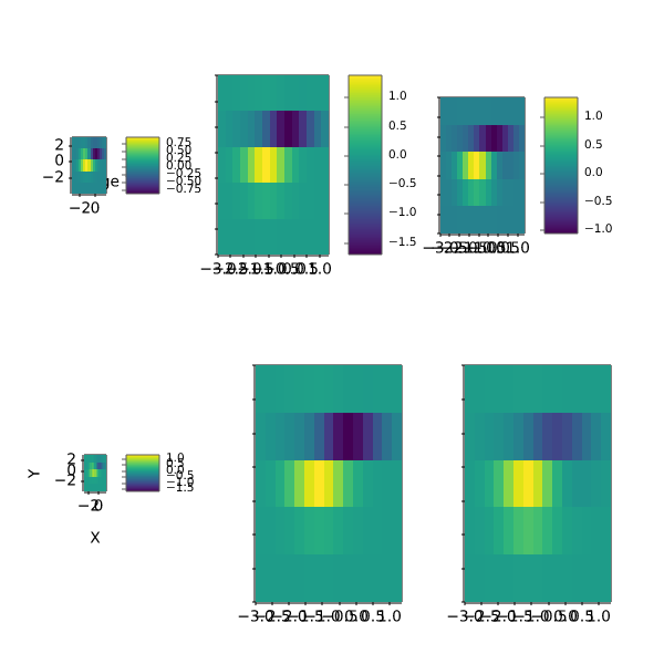
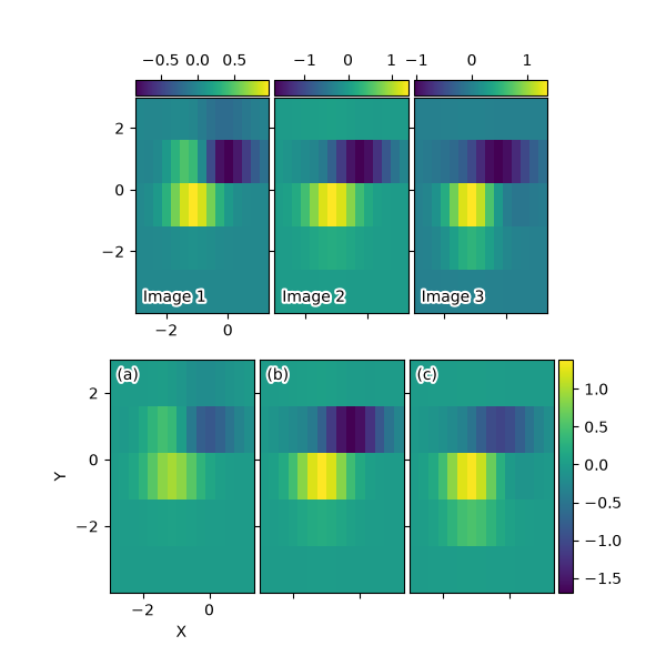
Grid of images with shared xaxis and yaxis.
"""

import matplotlib.pyplot as plt
import numpy as np

from matplotlib import cbook
from mpl_toolkits.axes_grid1 import ImageGrid


def add_inner_title(ax, title, loc, **kwargs):
    from matplotlib.offsetbox import AnchoredText
    from matplotlib.patheffects import withStroke
    prop = dict(path_effects=[withStroke(foreground='w', linewidth=3)],
                size=plt.rcParams['legend.fontsize'])
    at = AnchoredText(title, loc=loc, prop=prop,
                      pad=0., borderpad=0.5,
                      frameon=False, **kwargs)
    ax.add_artist(at)
    return at


fig = plt.figure(figsize=(6, 6))

# Prepare images
Z = cbook.get_sample_data("axes_grid/bivariate_normal.npy")
extent = (-3, 4, -4, 3)
ZS = [Z[i::3, :] for i in range(3)]
extent = extent[0], extent[1]/3., extent[2], extent[3]

# *** Demo 1: colorbar at each Axes ***
grid = ImageGrid(
    # 211 = at the position of fig.add_subplot(211)
    fig, 211, nrows_ncols=(1, 3), axes_pad=0.05, label_mode="1", share_all=True,
    cbar_location="top", cbar_mode="each", cbar_size="7%", cbar_pad="1%")
grid[0].set(xticks=[-2, 0], yticks=[-2, 0, 2])

for i, (ax, z) in enumerate(zip(grid, ZS)):
    im = ax.imshow(z, origin="lower", extent=extent)
    cb = ax.cax.colorbar(im)
    # Changing the colorbar ticks
    if i in [1, 2]:
        cb.set_ticks([-1, 0, 1])

for ax, im_title in zip(grid, ["Image 1", "Image 2", "Image 3"]):
    add_inner_title(ax, im_title, loc='lower left')

# *** Demo 2: shared colorbar ***
grid2 = ImageGrid(
    fig, 212, nrows_ncols=(1, 3), axes_pad=0.05, label_mode="1", share_all=True,
    cbar_location="right", cbar_mode="single", cbar_size="10%", cbar_pad=0.05)
grid2[0].set(xlabel="X", ylabel="Y", xticks=[-2, 0], yticks=[-2, 0, 2])

clim = (np.min(ZS), np.max(ZS))
for ax, z in zip(grid2, ZS):
    im = ax.imshow(z, clim=clim, origin="lower", extent=extent)

# With cbar_mode="single", cax attribute of all Axes are identical.
ax.cax.colorbar(im)

for ax, im_title in zip(grid2, ["(a)", "(b)", "(c)"]):
    add_inner_title(ax, im_title, loc='upper left')

plt.show()
axes_grid1/demo_axes_hbox_divider
================================
Source
"""
================================
HBoxDivider and VBoxDivider demo
================================

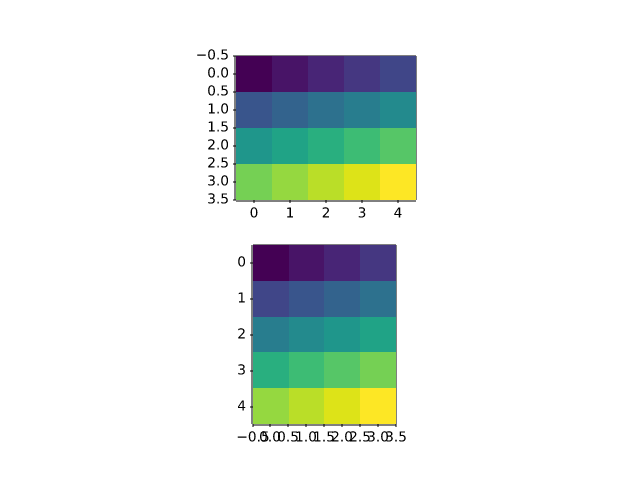
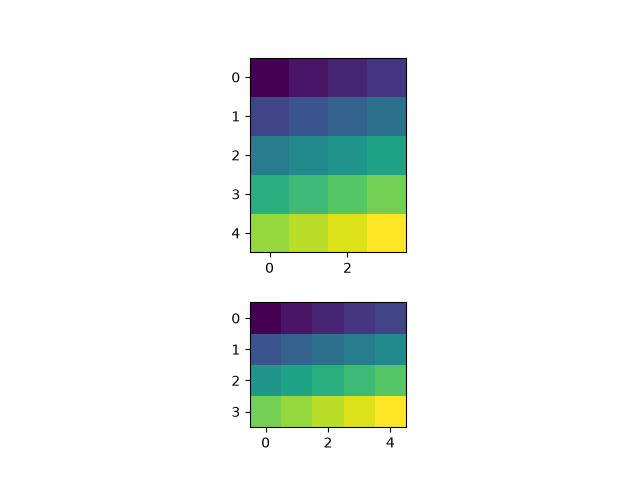
Using an `.HBoxDivider` to arrange subplots.

Note that both Axes' location are adjusted so that they have
equal heights while maintaining their aspect ratios.

"""

import matplotlib.pyplot as plt
import numpy as np

from mpl_toolkits.axes_grid1.axes_divider import HBoxDivider, VBoxDivider
import mpl_toolkits.axes_grid1.axes_size as Size

arr1 = np.arange(20).reshape((4, 5))
arr2 = np.arange(20).reshape((5, 4))

fig, (ax1, ax2) = plt.subplots(1, 2)
ax1.imshow(arr1)
ax2.imshow(arr2)

pad = 0.5  # pad in inches
divider = HBoxDivider(
    fig, 111,
    horizontal=[Size.AxesX(ax1), Size.Fixed(pad), Size.AxesX(ax2)],
    vertical=[Size.AxesY(ax1), Size.Scaled(1), Size.AxesY(ax2)])
ax1.set_axes_locator(divider.new_locator(0))
ax2.set_axes_locator(divider.new_locator(2))

plt.show()

# %%
# Using a `.VBoxDivider` to arrange subplots.
#
# Note that both Axes' location are adjusted so that they have
# equal widths while maintaining their aspect ratios.

fig, (ax1, ax2) = plt.subplots(2, 1)
ax1.imshow(arr1)
ax2.imshow(arr2)

divider = VBoxDivider(
    fig, 111,
    horizontal=[Size.AxesX(ax1), Size.Scaled(1), Size.AxesX(ax2)],
    vertical=[Size.AxesY(ax1), Size.Fixed(pad), Size.AxesY(ax2)])

ax1.set_axes_locator(divider.new_locator(0))
ax2.set_axes_locator(divider.new_locator(2))

plt.show()
axes_grid1/demo_axes_rgb
===============================
Source
"""
===============================
Show RGB channels using RGBAxes
===============================

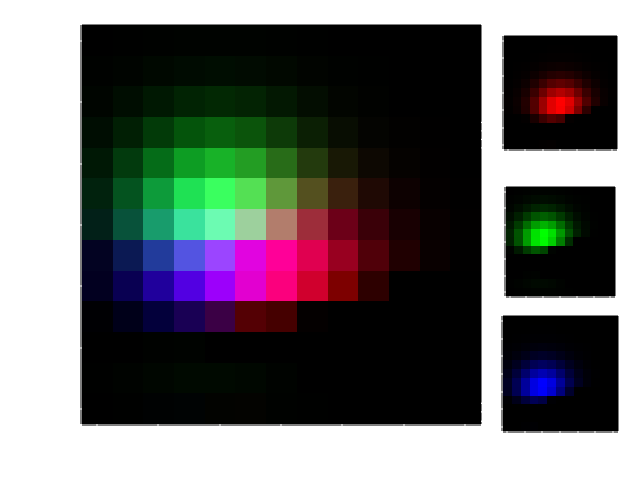
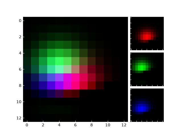
`~.axes_grid1.axes_rgb.RGBAxes` creates a layout of 4 Axes for displaying RGB
channels: one large Axes for the RGB image and 3 smaller Axes for the R, G, B
channels.
"""

import matplotlib.pyplot as plt
import numpy as np

from matplotlib import cbook
from mpl_toolkits.axes_grid1.axes_rgb import RGBAxes, make_rgb_axes


def get_rgb():
    Z = cbook.get_sample_data("axes_grid/bivariate_normal.npy")
    Z[Z < 0] = 0.
    Z = Z / Z.max()

    R = Z[:13, :13]
    G = Z[2:, 2:]
    B = Z[:13, 2:]

    return R, G, B


def make_cube(r, g, b):
    ny, nx = r.shape
    R = np.zeros((ny, nx, 3))
    R[:, :, 0] = r
    G = np.zeros_like(R)
    G[:, :, 1] = g
    B = np.zeros_like(R)
    B[:, :, 2] = b

    RGB = R + G + B

    return R, G, B, RGB


def demo_rgb1():
    fig = plt.figure()
    ax = RGBAxes(fig, [0.1, 0.1, 0.8, 0.8], pad=0.0)
    r, g, b = get_rgb()
    ax.imshow_rgb(r, g, b)


def demo_rgb2():
    fig, ax = plt.subplots()
    ax_r, ax_g, ax_b = make_rgb_axes(ax, pad=0.02)

    r, g, b = get_rgb()
    im_r, im_g, im_b, im_rgb = make_cube(r, g, b)
    ax.imshow(im_rgb)
    ax_r.imshow(im_r)
    ax_g.imshow(im_g)
    ax_b.imshow(im_b)

    for ax in fig.axes:
        ax.tick_params(direction='in', color='w')
        ax.spines[:].set_color("w")


demo_rgb1()
demo_rgb2()

plt.show()
axes_grid1/demo_colorbar_with_axes_divider
.. _demo-colorbar-with-axes-divider:
Source
"""
.. _demo-colorbar-with-axes-divider:

=========================
Colorbar with AxesDivider
=========================

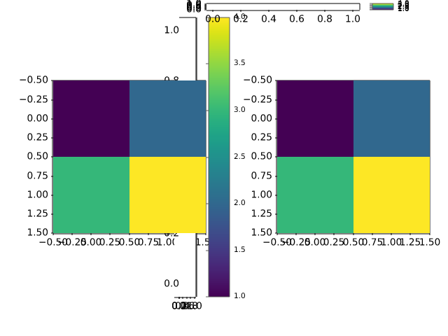
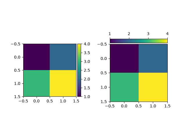
The `.axes_divider.make_axes_locatable` function takes an existing Axes, adds
it to a new `.AxesDivider` and returns the `.AxesDivider`.  The `.append_axes`
method of the `.AxesDivider` can then be used to create a new Axes on a given
side ("top", "right", "bottom", or "left") of the original Axes. This example
uses `.append_axes` to add colorbars next to Axes.

Users should consider simply passing the main Axes to the *ax* keyword argument of
`~.Figure.colorbar` instead of creating a locatable Axes manually like this.
See :ref:`colorbar_placement`.

.. redirect-from:: /gallery/axes_grid1/simple_colorbar
"""

import matplotlib.pyplot as plt

from mpl_toolkits.axes_grid1.axes_divider import make_axes_locatable

fig, (ax1, ax2) = plt.subplots(1, 2)
fig.subplots_adjust(wspace=0.5)

im1 = ax1.imshow([[1, 2], [3, 4]])
ax1_divider = make_axes_locatable(ax1)
# Add an Axes to the right of the main Axes.
cax1 = ax1_divider.append_axes("right", size="7%", pad="2%")
cb1 = fig.colorbar(im1, cax=cax1)

im2 = ax2.imshow([[1, 2], [3, 4]])
ax2_divider = make_axes_locatable(ax2)
# Add an Axes above the main Axes.
cax2 = ax2_divider.append_axes("top", size="7%", pad="2%")
cb2 = fig.colorbar(im2, cax=cax2, orientation="horizontal")
# Change tick position to top (with the default tick position "bottom", ticks
# overlap the image).
cax2.xaxis.set_ticks_position("top")

plt.show()
axes_grid1/demo_colorbar_with_inset_locator
.. _demo-colorbar-with-inset-locator:
Source
"""
.. _demo-colorbar-with-inset-locator:

=========================================================================
Control the position and size of a colorbar with inset_locator.inset_axes
=========================================================================

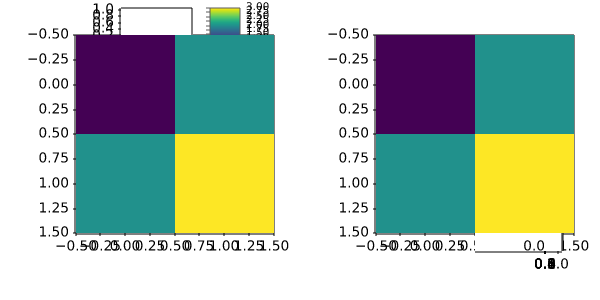
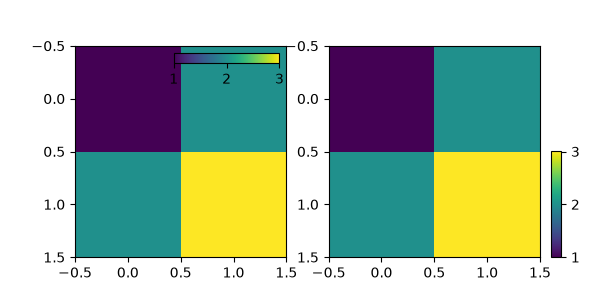
This example shows how to control the position, height, and width of colorbars
using `.inset_locator.inset_axes`.

`.inset_locator.inset_axes` placement is controlled as for legends: either
by providing a *loc* option ("upper right", "best", ...), or by providing a
locator with respect to the parent bbox.  Parameters such as *bbox_to_anchor*
and *borderpad* likewise work in the same way, and are also demonstrated here.

Users should consider using `.Axes.inset_axes` instead (see
:ref:`colorbar_placement`).

.. redirect-from:: /gallery/axes_grid1/demo_colorbar_of_inset_axes
"""

import matplotlib.pyplot as plt

from mpl_toolkits.axes_grid1 import inset_locator

fig, (ax1, ax2) = plt.subplots(1, 2, figsize=[6, 3])

im1 = ax1.imshow([[1, 2], [2, 3]])
axins1 = inset_locator.inset_axes(
    ax1,
    width="50%",  # width: 50% of parent_bbox width
    height="5%",  # height: 5%
    loc="upper right",
)
axins1.xaxis.set_ticks_position("bottom")
fig.colorbar(im1, cax=axins1, orientation="horizontal", ticks=[1, 2, 3])

im = ax2.imshow([[1, 2], [2, 3]])
axins = inset_locator.inset_axes(
    ax2,
    width="5%",  # width: 5% of parent_bbox width
    height="50%",  # height: 50%
    loc="lower left",
    bbox_to_anchor=(1.05, 0., 1, 1),
    bbox_transform=ax2.transAxes,
    borderpad=0,
)
fig.colorbar(im, cax=axins, ticks=[1, 2, 3])

plt.show()
axes_grid1/demo_edge_colorbar
===============================
Source
"""
===============================
Per-row or per-column colorbars
===============================

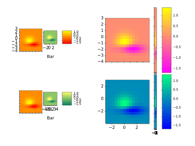
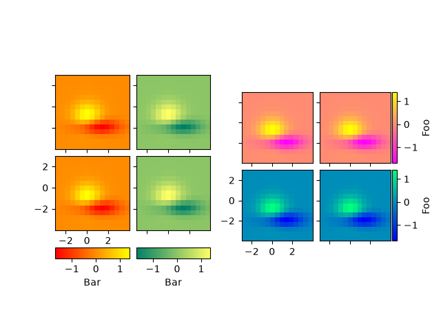
This example shows how to use one common colorbar for each row or column
of an image grid.
"""

import matplotlib.pyplot as plt

from matplotlib import cbook
from mpl_toolkits.axes_grid1 import AxesGrid


def get_demo_image():
    z = cbook.get_sample_data("axes_grid/bivariate_normal.npy")  # 15x15 array
    return z, (-3, 4, -4, 3)


def demo_bottom_cbar(fig):
    """
    A grid of 2x2 images with a colorbar for each column.
    """
    grid = AxesGrid(fig, 121,  # similar to subplot(121)
                    nrows_ncols=(2, 2),
                    axes_pad=0.10,
                    share_all=True,
                    label_mode="1",
                    cbar_location="bottom",
                    cbar_mode="edge",
                    cbar_pad=0.25,
                    cbar_size="15%",
                    direction="column"
                    )

    Z, extent = get_demo_image()
    cmaps = ["autumn", "summer"]
    for i in range(4):
        im = grid[i].imshow(Z, extent=extent, cmap=cmaps[i//2])
        if i % 2:
            grid.cbar_axes[i//2].colorbar(im)

    for cax in grid.cbar_axes:
        cax.axis[cax.orientation].set_label("Bar")

    # This affects all Axes as share_all = True.
    grid.axes_llc.set_xticks([-2, 0, 2])
    grid.axes_llc.set_yticks([-2, 0, 2])


def demo_right_cbar(fig):
    """
    A grid of 2x2 images. Each row has its own colorbar.
    """
    grid = AxesGrid(fig, 122,  # similar to subplot(122)
                    nrows_ncols=(2, 2),
                    axes_pad=0.10,
                    label_mode="1",
                    share_all=True,
                    cbar_location="right",
                    cbar_mode="edge",
                    cbar_size="7%",
                    cbar_pad="2%",
                    )
    Z, extent = get_demo_image()
    cmaps = ["spring", "winter"]
    for i in range(4):
        im = grid[i].imshow(Z, extent=extent, cmap=cmaps[i//2])
        if i % 2:
            grid.cbar_axes[i//2].colorbar(im)

    for cax in grid.cbar_axes:
        cax.axis[cax.orientation].set_label('Foo')

    # This affects all Axes because we set share_all = True.
    grid.axes_llc.set_xticks([-2, 0, 2])
    grid.axes_llc.set_yticks([-2, 0, 2])


fig = plt.figure()

demo_bottom_cbar(fig)
demo_right_cbar(fig)

plt.show()
axes_grid1/demo_fixed_size_axes
===============================
Source
"""
===============================
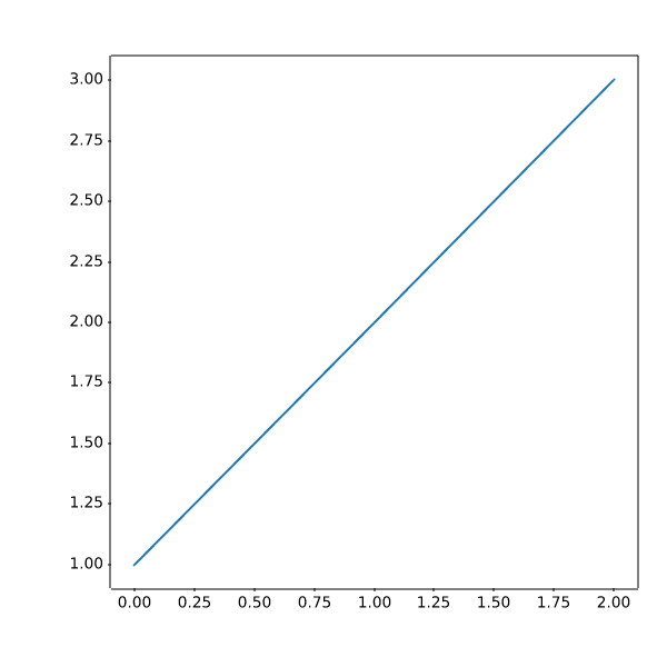
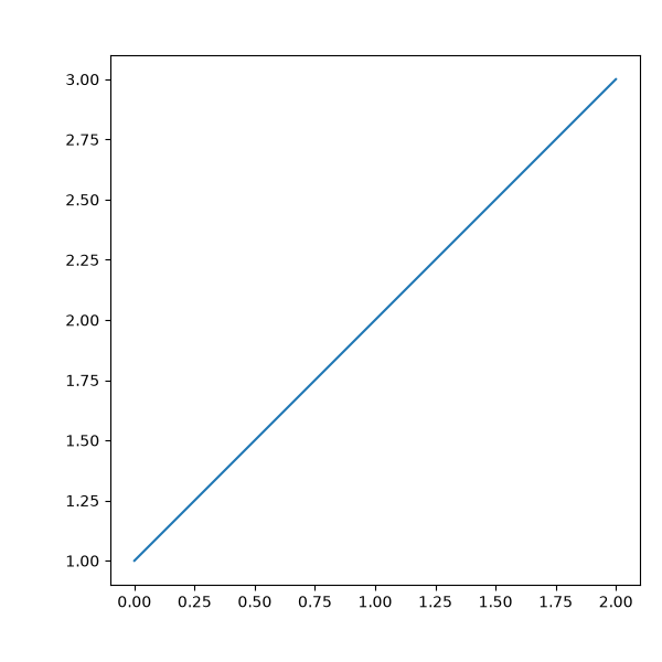
Axes with a fixed physical size
===============================

Note that this can be accomplished with the main library for
Axes on Figures that do not change size: :ref:`fixed_size_axes`
"""

import matplotlib.pyplot as plt

from mpl_toolkits.axes_grid1 import Divider, Size

# %%


fig = plt.figure(figsize=(6, 6))

# The first items are for padding and the second items are for the Axes.
# sizes are in inch.
h = [Size.Fixed(1.0), Size.Fixed(4.5)]
v = [Size.Fixed(0.7), Size.Fixed(5.)]

divider = Divider(fig, (0, 0, 1, 1), h, v, aspect=False)
# The width and height of the rectangle are ignored.

ax = fig.add_axes(divider.get_position(),
                  axes_locator=divider.new_locator(nx=1, ny=1))

ax.plot([1, 2, 3])

# %%


fig = plt.figure(figsize=(6, 6))

# The first & third items are for padding and the second items are for the
# Axes. Sizes are in inches.
h = [Size.Fixed(1.0), Size.Scaled(1.), Size.Fixed(.2)]
v = [Size.Fixed(0.7), Size.Scaled(1.), Size.Fixed(.5)]

divider = Divider(fig, (0, 0, 1, 1), h, v, aspect=False)
# The width and height of the rectangle are ignored.

ax = fig.add_axes(divider.get_position(),
                  axes_locator=divider.new_locator(nx=1, ny=1))

ax.plot([1, 2, 3])

plt.show()
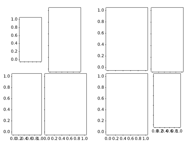
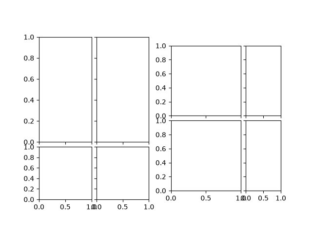
axes_grid1/demo_imagegrid_aspect
=========================================
Source
"""
=========================================
ImageGrid cells with a fixed aspect ratio
=========================================
"""

import matplotlib.pyplot as plt

from mpl_toolkits.axes_grid1 import ImageGrid

fig = plt.figure()

grid1 = ImageGrid(fig, 121, (2, 2), axes_pad=0.1,
                  aspect=True, share_all=True)
for i in [0, 1]:
    grid1[i].set_aspect(2)

grid2 = ImageGrid(fig, 122, (2, 2), axes_pad=0.1,
                  aspect=True, share_all=True)
for i in [1, 3]:
    grid2[i].set_aspect(2)

plt.show()
axes_grid1/inset_locator_demo
==================
Source
"""
==================
Inset locator demo
==================

"""

# %%
# The `.inset_locator`'s `~.inset_locator.inset_axes` allows
# easily placing insets in the corners of the Axes by specifying a width and
# height and optionally a location (loc) that accepts locations as codes,
# similar to `~matplotlib.axes.Axes.legend`.
# By default, the inset is offset by some points from the axes,
# controlled via the *borderpad* parameter.

import matplotlib.pyplot as plt

from mpl_toolkits.axes_grid1.inset_locator import inset_axes

fig, (ax, ax2) = plt.subplots(1, 2, figsize=[5.5, 2.8])

# Create inset of width 1.3 inches and height 0.9 inches
# at the default upper right location.
axins = inset_axes(ax, width=1.3, height=0.9)

# Create inset of width 30% and height 40% of the parent Axes' bounding box
# at the lower left corner.
axins2 = inset_axes(ax, width="30%", height="40%", loc="lower left")

# Create inset of mixed specifications in the second subplot;
# width is 30% of parent Axes' bounding box and
# height is 1 inch at the upper left corner.
axins3 = inset_axes(ax2, width="30%", height=1., loc="upper left")

# Create an inset in the lower right corner with borderpad=1, i.e.
# 10 points padding (as 10pt is the default fontsize) to the parent Axes.
axins4 = inset_axes(ax2, width="20%", height="20%", loc="lower right", borderpad=1)

# Turn ticklabels of insets off
for axi in [axins, axins2, axins3, axins4]:
    axi.tick_params(labelleft=False, labelbottom=False)

plt.show()


# %%
# The parameters *bbox_to_anchor* and *bbox_transform* can be used for a more
# fine-grained control over the inset position and size or even to position
# the inset at completely arbitrary positions.
# The *bbox_to_anchor* sets the bounding box in coordinates according to the
# *bbox_transform*.
#

fig = plt.figure(figsize=[5.5, 2.8])
ax = fig.add_subplot(121)

# We use the Axes transform as bbox_transform. Therefore, the bounding box
# needs to be specified in axes coordinates ((0, 0) is the lower left corner
# of the Axes, (1, 1) is the upper right corner).
# The bounding box (.2, .4, .6, .5) starts at (.2, .4) and ranges to (.8, .9)
# in those coordinates.
# Inside this bounding box an inset of half the bounding box' width and
# three quarters of the bounding box' height is created. The lower left corner
# of the inset is aligned to the lower left corner of the bounding box.
# The inset is then offset by the default 0.5 in units of the font size.

axins = inset_axes(ax, width="50%", height="75%",
                   bbox_to_anchor=(.2, .4, .6, .5),
                   bbox_transform=ax.transAxes, loc="lower left")

# For visualization purposes we mark the bounding box by a rectangle
ax.add_patch(plt.Rectangle((.2, .4), .6, .5, ls="--", ec="c", fc="none",
                           transform=ax.transAxes))

# We set the axis limits to something other than the default, in order to not
# distract from the fact that axes coordinates are used here.
ax.set(xlim=(0, 10), ylim=(0, 10))


# Note how the two following insets are created at the same positions, one by
# use of the default parent Axes' bbox and the other via a bbox in Axes
# coordinates and the respective transform.
ax2 = fig.add_subplot(222)
axins2 = inset_axes(ax2, width="30%", height="50%")

ax3 = fig.add_subplot(224)
axins3 = inset_axes(ax3, width="100%", height="100%",
                    bbox_to_anchor=(.7, .5, .3, .5),
                    bbox_transform=ax3.transAxes)

# For visualization purposes we mark the bounding box by a rectangle
ax2.add_patch(plt.Rectangle((0, 0), 1, 1, ls="--", lw=2, ec="c", fc="none"))
ax3.add_patch(plt.Rectangle((.7, .5), .3, .5, ls="--", lw=2,
                            ec="c", fc="none"))

# Turn ticklabels off
for axi in [axins2, axins3, ax2, ax3]:
    axi.tick_params(labelleft=False, labelbottom=False)

plt.show()


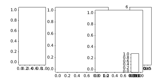
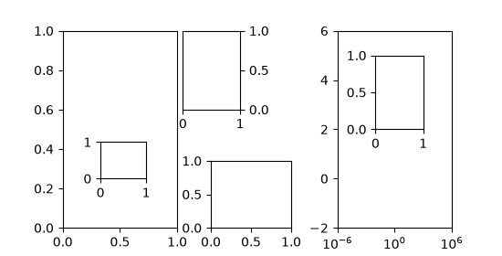
# %%
# In the above the Axes transform together with 4-tuple bounding boxes has been
# used as it mostly is useful to specify an inset relative to the Axes it is
# an inset to. However, other use cases are equally possible. The following
# example examines some of those.
#

fig = plt.figure(figsize=[5.5, 2.8])
ax = fig.add_subplot(131)

# Create an inset outside the Axes
axins = inset_axes(ax, width="100%", height="100%",
                   bbox_to_anchor=(1.05, .6, .5, .4),
                   bbox_transform=ax.transAxes, loc="upper left", borderpad=0)
axins.tick_params(left=False, right=True, labelleft=False, labelright=True)

# Create an inset with a 2-tuple bounding box. Note that this creates a
# bbox without extent. This hence only makes sense when specifying
# width and height in absolute units (inches).
axins2 = inset_axes(ax, width=0.5, height=0.4,
                    bbox_to_anchor=(0.33, 0.25),
                    bbox_transform=ax.transAxes, loc="lower left", borderpad=0)


ax2 = fig.add_subplot(133)
ax2.set_xscale("log")
ax2.set(xlim=(1e-6, 1e6), ylim=(-2, 6))

# Create inset in data coordinates using ax.transData as transform
axins3 = inset_axes(ax2, width="100%", height="100%",
                    bbox_to_anchor=(1e-2, 2, 1e3, 3),
                    bbox_transform=ax2.transData, loc="upper left", borderpad=0)

# Create an inset horizontally centered in figure coordinates and vertically
# bound to line up with the Axes.
from matplotlib.transforms import blended_transform_factory  # noqa

transform = blended_transform_factory(fig.transFigure, ax2.transAxes)
axins4 = inset_axes(ax2, width="16%", height="34%",
                    bbox_to_anchor=(0, 0, 1, 1),
                    bbox_transform=transform, loc="lower center", borderpad=0)

plt.show()
axes_grid1/inset_locator_demo2
====================
Source
"""
====================
Inset locator demo 2
====================

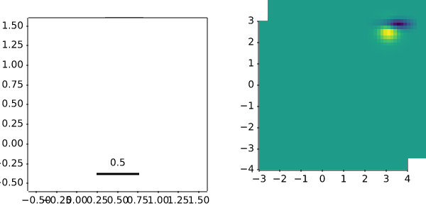
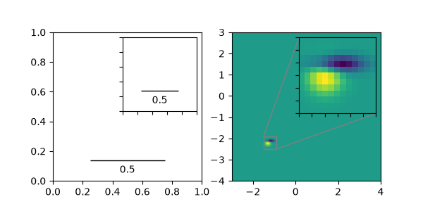
This demo shows how to create a zoomed inset via `.zoomed_inset_axes`.
In the first subplot an `.AnchoredSizeBar` shows the zoom effect.
In the second subplot a connection to the region of interest is
created via `.mark_inset`.

A version of the second subplot, not using the toolkit, is available in
:doc:`/gallery/subplots_axes_and_figures/zoom_inset_axes`.
"""

import matplotlib.pyplot as plt
import numpy as np

from matplotlib import cbook
from mpl_toolkits.axes_grid1.anchored_artists import AnchoredSizeBar
from mpl_toolkits.axes_grid1.inset_locator import mark_inset, zoomed_inset_axes

fig, (ax, ax2) = plt.subplots(ncols=2, figsize=[6, 3])


# First subplot, showing an inset with a size bar.
ax.set_aspect(1)

axins = zoomed_inset_axes(ax, zoom=0.5, loc='upper right')
# fix the number of ticks on the inset Axes
axins.yaxis.get_major_locator().set_params(nbins=7)
axins.xaxis.get_major_locator().set_params(nbins=7)
axins.tick_params(labelleft=False, labelbottom=False)


def add_sizebar(ax, size):
    asb = AnchoredSizeBar(ax.transData,
                          size,
                          str(size),
                          loc="lower center",
                          pad=0.1, borderpad=0.5, sep=5,
                          frameon=False)
    ax.add_artist(asb)

add_sizebar(ax, 0.5)
add_sizebar(axins, 0.5)


# Second subplot, showing an image with an inset zoom and a marked inset
Z = cbook.get_sample_data("axes_grid/bivariate_normal.npy")  # 15x15 array
extent = (-3, 4, -4, 3)
Z2 = np.zeros((150, 150))
ny, nx = Z.shape
Z2[30:30+ny, 30:30+nx] = Z

ax2.imshow(Z2, extent=extent, origin="lower")

axins2 = zoomed_inset_axes(ax2, zoom=6, loc="upper right")
axins2.imshow(Z2, extent=extent, origin="lower")

# subregion of the original image
x1, x2, y1, y2 = -1.5, -0.9, -2.5, -1.9
axins2.set_xlim(x1, x2)
axins2.set_ylim(y1, y2)
# fix the number of ticks on the inset Axes
axins2.yaxis.get_major_locator().set_params(nbins=7)
axins2.xaxis.get_major_locator().set_params(nbins=7)
axins2.tick_params(labelleft=False, labelbottom=False)

# draw a bbox of the region of the inset Axes in the parent Axes and
# connecting lines between the bbox and the inset Axes area
mark_inset(ax2, axins2, loc1=2, loc2=4, fc="none", ec="0.5")

plt.show()
axes_grid1/make_room_for_ylabel_using_axesgrid
====================================
Source
"""
====================================
Make room for ylabel using axes_grid
====================================
"""

import matplotlib.pyplot as plt

from mpl_toolkits.axes_grid1 import make_axes_locatable
from mpl_toolkits.axes_grid1.axes_divider import make_axes_area_auto_adjustable

fig = plt.figure()
ax = fig.add_axes((0, 0, 1, 1))

ax.set_yticks([0.5], labels=["very long label"])

make_axes_area_auto_adjustable(ax)

# %%

fig = plt.figure()
ax1 = fig.add_axes((0, 0, 1, 0.5))
ax2 = fig.add_axes((0, 0.5, 1, 0.5))

ax1.set_yticks([0.5], labels=["very long label"])
ax1.set_ylabel("Y label")

ax2.set_title("Title")

make_axes_area_auto_adjustable(ax1, pad=0.1, use_axes=[ax1, ax2])
make_axes_area_auto_adjustable(ax2, pad=0.1, use_axes=[ax1, ax2])

# %%

fig = plt.figure()
ax1 = fig.add_axes((0, 0, 1, 1))
divider = make_axes_locatable(ax1)

ax2 = divider.append_axes("right", "100%", pad=0.3, sharey=ax1)
ax2.tick_params(labelleft=False)
fig.add_axes(ax2)

divider.add_auto_adjustable_area(use_axes=[ax1], pad=0.1,
                                 adjust_dirs=["left"])
divider.add_auto_adjustable_area(use_axes=[ax2], pad=0.1,
                                 adjust_dirs=["right"])
divider.add_auto_adjustable_area(use_axes=[ax1, ax2], pad=0.1,
                                 adjust_dirs=["top", "bottom"])

ax1.set_yticks([0.5], labels=["very long label"])

ax2.set_title("Title")
ax2.set_xlabel("X - Label")

plt.show()
axes_grid1/parasite_simple
===============
Source
"""
===============
Parasite Simple
===============
"""

import matplotlib.pyplot as plt

from mpl_toolkits.axes_grid1 import host_subplot

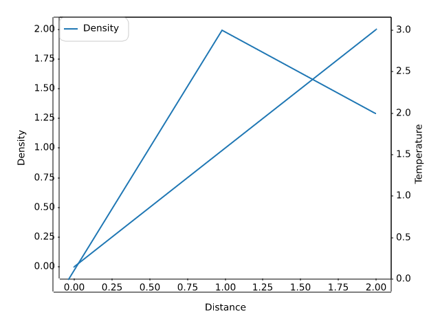
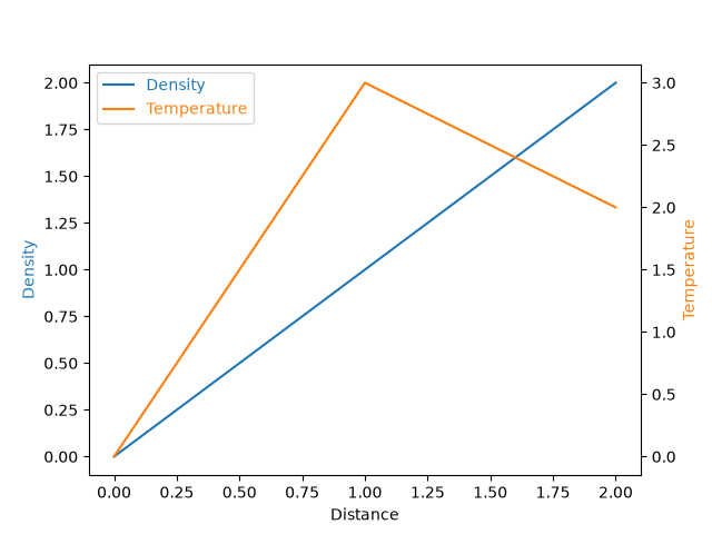
host = host_subplot(111)
par = host.twinx()

host.set_xlabel("Distance")
host.set_ylabel("Density")
par.set_ylabel("Temperature")

p1, = host.plot([0, 1, 2], [0, 1, 2], label="Density")
p2, = par.plot([0, 1, 2], [0, 3, 2], label="Temperature")

host.legend(labelcolor="linecolor")

host.yaxis.label.set_color(p1.get_color())
par.yaxis.label.set_color(p2.get_color())

plt.show()
axes_grid1/parasite_simple2
================
Source
"""
================
Parasite Simple2
================

"""
import matplotlib.pyplot as plt

import matplotlib.transforms as mtransforms
from mpl_toolkits.axes_grid1.parasite_axes import HostAxes

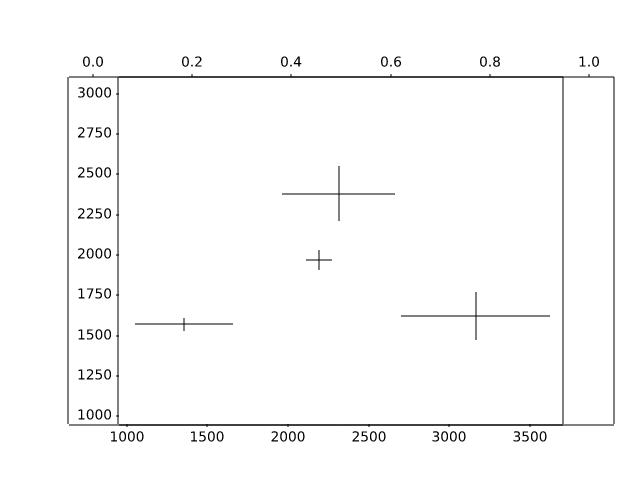
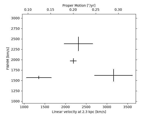
obs = [["01_S1", 3.88, 0.14, 1970, 63],
       ["01_S4", 5.6, 0.82, 1622, 150],
       ["02_S1", 2.4, 0.54, 1570, 40],
       ["03_S1", 4.1, 0.62, 2380, 170]]


fig = plt.figure()

ax_kms = fig.add_subplot(axes_class=HostAxes, aspect=1)

# angular proper motion("/yr) to linear velocity(km/s) at distance=2.3kpc
pm_to_kms = 1./206265.*2300*3.085e18/3.15e7/1.e5

aux_trans = mtransforms.Affine2D().scale(pm_to_kms, 1.)
ax_pm = ax_kms.twin(aux_trans)

for n, ds, dse, w, we in obs:
    time = ((2007 + (10. + 4/30.)/12) - 1988.5)
    v = ds / time * pm_to_kms
    ve = dse / time * pm_to_kms
    ax_kms.errorbar([v], [w], xerr=[ve], yerr=[we], color="k")


ax_kms.axis["bottom"].set_label("Linear velocity at 2.3 kpc [km/s]")
ax_kms.axis["left"].set_label("FWHM [km/s]")
ax_pm.axis["top"].set_label(r"Proper Motion [$''$/yr]")
ax_pm.axis["top"].label.set_visible(True)
ax_pm.axis["right"].major_ticklabels.set_visible(False)

ax_kms.set_xlim(950, 3700)
ax_kms.set_ylim(950, 3100)
# xlim and ylim of ax_pms will be automatically adjusted.

plt.show()
axes_grid1/scatter_hist_locatable_axes
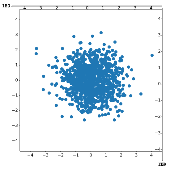
====================================================
Source
"""
====================================================
Align histogram to scatter plot using locatable Axes
====================================================

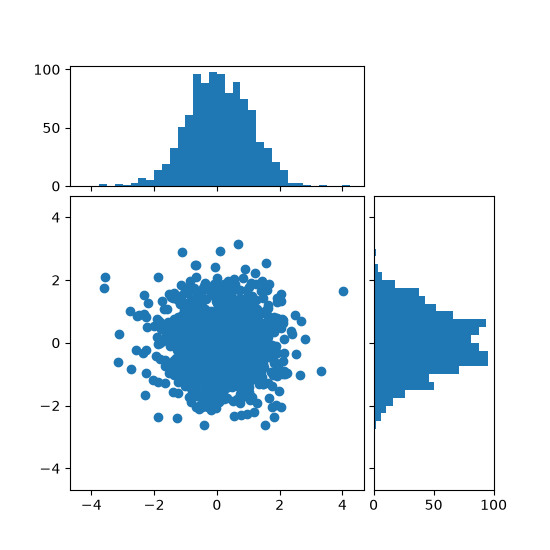
Show the marginal distributions of a scatter plot as histograms at the sides of
the plot.

For a nice alignment of the main Axes with the marginals, the Axes positions
are defined by a ``Divider``, produced via `.make_axes_locatable`.  Note that
the ``Divider`` API allows setting Axes sizes and pads in inches, which is its
main feature.

If one wants to set Axes sizes and pads relative to the main Figure, see the
:doc:`/gallery/lines_bars_and_markers/scatter_hist` example.
"""

import matplotlib.pyplot as plt
import numpy as np

from mpl_toolkits.axes_grid1 import make_axes_locatable

# Fixing random state for reproducibility
np.random.seed(19680801)

# the random data
x = np.random.randn(1000)
y = np.random.randn(1000)


fig, ax = plt.subplots(figsize=(5.5, 5.5))

# the scatter plot:
ax.scatter(x, y)

# Set aspect of the main Axes.
ax.set_aspect(1.)

# create new Axes on the right and on the top of the current Axes
divider = make_axes_locatable(ax)
# below height and pad are in inches
ax_histx = divider.append_axes("top", 1.2, pad=0.1, sharex=ax)
ax_histy = divider.append_axes("right", 1.2, pad=0.1, sharey=ax)

# make some labels invisible
ax_histx.xaxis.set_tick_params(labelbottom=False)
ax_histy.yaxis.set_tick_params(labelleft=False)

# now determine nice limits by hand:
binwidth = 0.25
xymax = max(np.max(np.abs(x)), np.max(np.abs(y)))
lim = (int(xymax/binwidth) + 1)*binwidth

bins = np.arange(-lim, lim + binwidth, binwidth)
ax_histx.hist(x, bins=bins)
ax_histy.hist(y, bins=bins, orientation='horizontal')

# the xaxis of ax_histx and yaxis of ax_histy are shared with ax,
# thus there is no need to manually adjust the xlim and ylim of these
# axis.

ax_histx.set_yticks([0, 50, 100])
ax_histy.set_xticks([0, 50, 100])

plt.show()

# %%
#
# .. admonition:: References
#
#    The use of the following functions, methods, classes and modules is shown
#    in this example:
#
#    - `mpl_toolkits.axes_grid1.axes_divider.make_axes_locatable`
#    - `matplotlib.axes.Axes.set_aspect`
#    - `matplotlib.axes.Axes.scatter`
#    - `matplotlib.axes.Axes.hist`
axes_grid1/simple_anchored_artists
=======================
Source
"""
=======================
Simple Anchored Artists
=======================

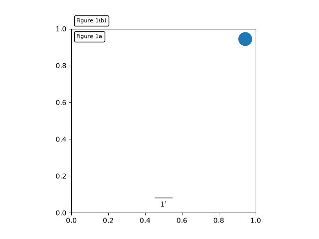
This example illustrates the use of the anchored helper classes found in
:mod:`matplotlib.offsetbox` and in :mod:`mpl_toolkits.axes_grid1`.
An implementation of a similar figure, but without use of the toolkit,
can be found in :doc:`/gallery/misc/anchored_artists`.
"""

import matplotlib.pyplot as plt


def draw_text(ax):
    """
    Draw two text-boxes, anchored by different corners to the upper-left
    corner of the figure.
    """
    from matplotlib.offsetbox import AnchoredText
    at = AnchoredText("Figure 1a",
                      loc='upper left', prop=dict(size=8), frameon=True,
                      )
    at.patch.set_boxstyle("round,pad=0.,rounding_size=0.2")
    ax.add_artist(at)

    at2 = AnchoredText("Figure 1(b)",
                       loc='lower left', prop=dict(size=8), frameon=True,
                       bbox_to_anchor=(0., 1.),
                       bbox_transform=ax.transAxes
                       )
    at2.patch.set_boxstyle("round,pad=0.,rounding_size=0.2")
    ax.add_artist(at2)


def draw_circle(ax):
    """
    Draw a circle in axis coordinates
    """
    from matplotlib.patches import Circle
    from mpl_toolkits.axes_grid1.anchored_artists import AnchoredDrawingArea
    ada = AnchoredDrawingArea(20, 20, 0, 0,
                              loc='upper right', pad=0., frameon=False)
    p = Circle((10, 10), 10)
    ada.da.add_artist(p)
    ax.add_artist(ada)


def draw_sizebar(ax):
    """
    Draw a horizontal bar with length of 0.1 in data coordinates,
    with a fixed label underneath.
    """
    from mpl_toolkits.axes_grid1.anchored_artists import AnchoredSizeBar
    asb = AnchoredSizeBar(ax.transData,
                          0.1,
                          r"1$^{\prime}$",
                          loc='lower center',
                          pad=0.1, borderpad=0.5, sep=5,
                          frameon=False)
    ax.add_artist(asb)


fig, ax = plt.subplots()
ax.set_aspect(1.)

draw_text(ax)
draw_circle(ax)
draw_sizebar(ax)

plt.show()
axes_grid1/simple_axes_divider1
=====================
Source
"""
=====================
Simple Axes Divider 1
=====================

See also :ref:`axes_grid`.
"""

import matplotlib.pyplot as plt

from mpl_toolkits.axes_grid1 import Divider, Size


def label_axes(ax, text):
    """Place a label at the center of an Axes, and remove the axis ticks."""
    ax.text(.5, .5, text, transform=ax.transAxes,
            horizontalalignment="center", verticalalignment="center")
    ax.tick_params(bottom=False, labelbottom=False,
                   left=False, labelleft=False)


# %%
# Fixed Axes sizes; fixed paddings.

fig = plt.figure(figsize=(6, 6))
fig.suptitle("Fixed axes sizes, fixed paddings")

# Sizes are in inches.
horiz = [Size.Fixed(1.), Size.Fixed(.5), Size.Fixed(1.5), Size.Fixed(.5)]
vert = [Size.Fixed(1.5), Size.Fixed(.5), Size.Fixed(1.)]

rect = (0.1, 0.1, 0.8, 0.8)
# Divide the Axes rectangle into a grid with sizes specified by horiz * vert.
div = Divider(fig, rect, horiz, vert, aspect=False)

# The rect parameter will actually be ignored and overridden by axes_locator.
ax1 = fig.add_axes(rect, axes_locator=div.new_locator(nx=0, ny=0))
label_axes(ax1, "nx=0, ny=0")
ax2 = fig.add_axes(rect, axes_locator=div.new_locator(nx=0, ny=2))
label_axes(ax2, "nx=0, ny=2")
ax3 = fig.add_axes(rect, axes_locator=div.new_locator(nx=2, ny=2))
label_axes(ax3, "nx=2, ny=2")
ax4 = fig.add_axes(rect, axes_locator=div.new_locator(nx=2, nx1=4, ny=0))
label_axes(ax4, "nx=2, nx1=4, ny=0")

# %%
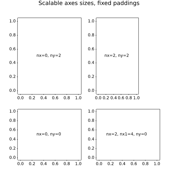
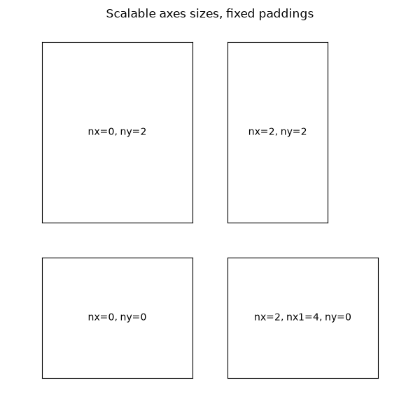
# Axes sizes that scale with the figure size; fixed paddings.

fig = plt.figure(figsize=(6, 6))
fig.suptitle("Scalable axes sizes, fixed paddings")

horiz = [Size.Scaled(1.5), Size.Fixed(.5), Size.Scaled(1.), Size.Scaled(.5)]
vert = [Size.Scaled(1.), Size.Fixed(.5), Size.Scaled(1.5)]

rect = (0.1, 0.1, 0.8, 0.8)
# Divide the Axes rectangle into a grid with sizes specified by horiz * vert.
div = Divider(fig, rect, horiz, vert, aspect=False)

# The rect parameter will actually be ignored and overridden by axes_locator.
ax1 = fig.add_axes(rect, axes_locator=div.new_locator(nx=0, ny=0))
label_axes(ax1, "nx=0, ny=0")
ax2 = fig.add_axes(rect, axes_locator=div.new_locator(nx=0, ny=2))
label_axes(ax2, "nx=0, ny=2")
ax3 = fig.add_axes(rect, axes_locator=div.new_locator(nx=2, ny=2))
label_axes(ax3, "nx=2, ny=2")
ax4 = fig.add_axes(rect, axes_locator=div.new_locator(nx=2, nx1=4, ny=0))
label_axes(ax4, "nx=2, nx1=4, ny=0")

plt.show()
axes_grid1/simple_axes_divider3
=====================
Source
"""
=====================
Simple axes divider 3
=====================

See also :ref:`axes_grid`.
"""

import matplotlib.pyplot as plt

from mpl_toolkits.axes_grid1 import Divider
import mpl_toolkits.axes_grid1.axes_size as Size

fig = plt.figure(figsize=(5.5, 4))

# the rect parameter will be ignored as we will set axes_locator
rect = (0.1, 0.1, 0.8, 0.8)
ax = [fig.add_axes(rect, label="%d" % i) for i in range(4)]


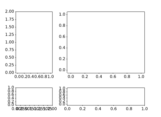
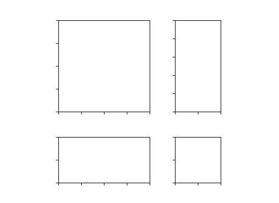
horiz = [Size.AxesX(ax[0]), Size.Fixed(.5), Size.AxesX(ax[1])]
vert = [Size.AxesY(ax[0]), Size.Fixed(.5), Size.AxesY(ax[2])]

# divide the Axes rectangle into grid whose size is specified by horiz * vert
divider = Divider(fig, rect, horiz, vert, aspect=False)


ax[0].set_axes_locator(divider.new_locator(nx=0, ny=0))
ax[1].set_axes_locator(divider.new_locator(nx=2, ny=0))
ax[2].set_axes_locator(divider.new_locator(nx=0, ny=2))
ax[3].set_axes_locator(divider.new_locator(nx=2, ny=2))

ax[0].set_xlim(0, 2)
ax[1].set_xlim(0, 1)

ax[0].set_ylim(0, 1)
ax[2].set_ylim(0, 2)

divider.set_aspect(1.)

for ax1 in ax:
    ax1.tick_params(labelbottom=False, labelleft=False)

plt.show()
axes_grid1/simple_axesgrid
================
Source
"""
================
Simple ImageGrid
================

Align multiple images using `~mpl_toolkits.axes_grid1.axes_grid.ImageGrid`.
"""

import matplotlib.pyplot as plt
import numpy as np

from mpl_toolkits.axes_grid1 import ImageGrid

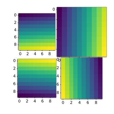
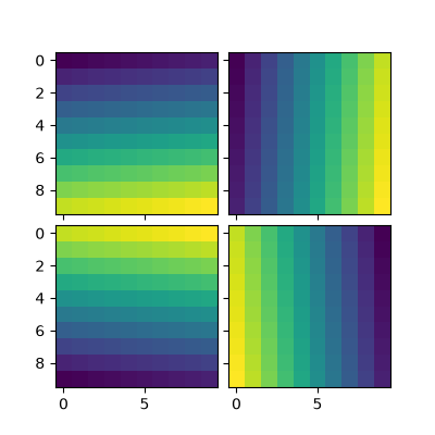
im1 = np.arange(100).reshape((10, 10))
im2 = im1.T
im3 = np.flipud(im1)
im4 = np.fliplr(im2)

fig = plt.figure(figsize=(4., 4.))
grid = ImageGrid(fig, 111,  # similar to subplot(111)
                 nrows_ncols=(2, 2),  # creates 2x2 grid of Axes
                 axes_pad=0.1,  # pad between Axes in inch.
                 )

for ax, im in zip(grid, [im1, im2, im3, im4]):
    # Iterating over the grid returns the Axes.
    ax.imshow(im)

plt.show()
axes_grid1/simple_axesgrid2
==================
Source
"""
==================
Simple ImageGrid 2
==================

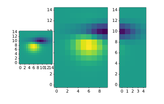
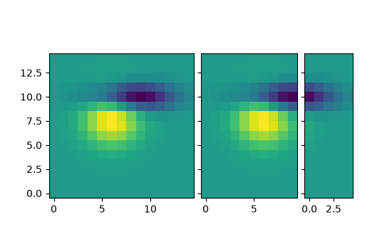
Align multiple images of different sizes using
`~mpl_toolkits.axes_grid1.axes_grid.ImageGrid`.
"""

import matplotlib.pyplot as plt

from matplotlib import cbook
from mpl_toolkits.axes_grid1 import ImageGrid

fig = plt.figure(figsize=(5.5, 3.5))
grid = ImageGrid(fig, 111,  # similar to subplot(111)
                 nrows_ncols=(1, 3),
                 axes_pad=0.1,
                 label_mode="L",
                 )

# demo image
Z = cbook.get_sample_data("axes_grid/bivariate_normal.npy")
im1 = Z
im2 = Z[:, :10]
im3 = Z[:, 10:]
vmin, vmax = Z.min(), Z.max()
for ax, im in zip(grid, [im1, im2, im3]):
    ax.imshow(im, origin="lower", vmin=vmin, vmax=vmax)

plt.show()
axes_grid1/simple_axisline4
================
Source
"""
================
Simple Axisline4
================

"""
import matplotlib.pyplot as plt
import numpy as np

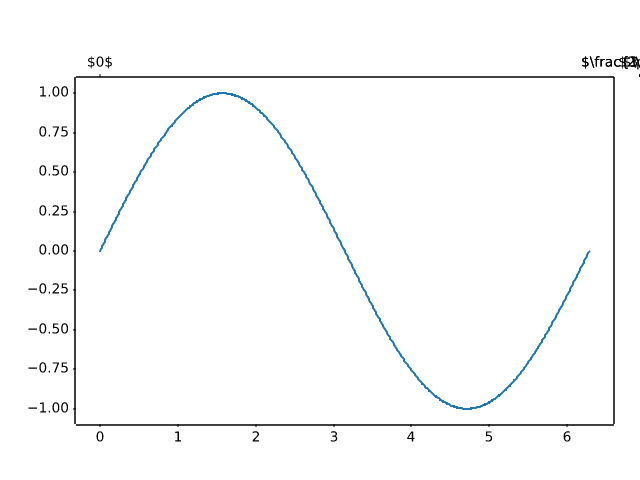
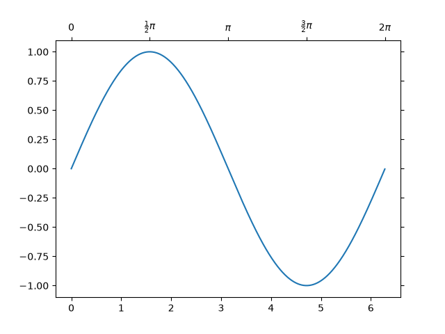
from mpl_toolkits.axes_grid1 import host_subplot

ax = host_subplot(111)
xx = np.arange(0, 2*np.pi, 0.01)
ax.plot(xx, np.sin(xx))

ax2 = ax.twin()  # ax2 is responsible for "top" axis and "right" axis
ax2.set_xticks([0., .5*np.pi, np.pi, 1.5*np.pi, 2*np.pi],
               labels=["$0$", r"$\frac{1}{2}\pi$",
                       r"$\pi$", r"$\frac{3}{2}\pi$", r"$2\pi$"])

ax2.axis["right"].major_ticklabels.set_visible(False)
ax2.axis["top"].major_ticklabels.set_visible(True)

plt.show()
axisartist/axis_direction
==============
Source
"""
==============
Axis Direction
==============
"""

import matplotlib.pyplot as plt

import mpl_toolkits.axisartist as axisartist


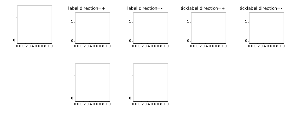
def setup_axes(fig, pos):
    ax = fig.add_subplot(pos, axes_class=axisartist.Axes)

    ax.set_ylim(-0.1, 1.5)
    ax.set_yticks([0, 1])

    ax.axis[:].set_visible(False)

    ax.axis["x"] = ax.new_floating_axis(1, 0.5)
    ax.axis["x"].set_axisline_style("->", size=1.5)

    return ax


plt.rcParams.update({
    "axes.titlesize": "medium",
    "axes.titley": 1.1,
})

fig = plt.figure(figsize=(10, 4))
fig.subplots_adjust(bottom=0.1, top=0.9, left=0.05, right=0.95)

ax1 = setup_axes(fig, 251)
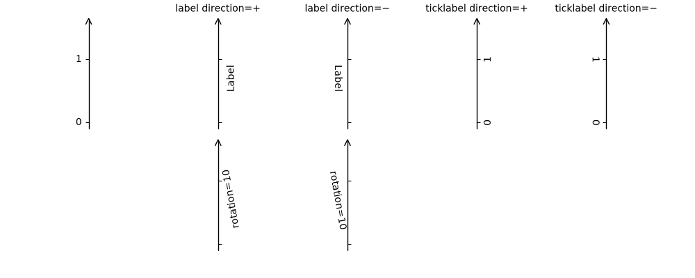
ax1.axis["x"].set_axis_direction("left")

ax2 = setup_axes(fig, 252)
ax2.axis["x"].label.set_text("Label")
ax2.axis["x"].toggle(ticklabels=False)
ax2.axis["x"].set_axislabel_direction("+")
ax2.set_title("label direction=$+$")

ax3 = setup_axes(fig, 253)
ax3.axis["x"].label.set_text("Label")
ax3.axis["x"].toggle(ticklabels=False)
ax3.axis["x"].set_axislabel_direction("-")
ax3.set_title("label direction=$-$")

ax4 = setup_axes(fig, 254)
ax4.axis["x"].set_ticklabel_direction("+")
ax4.set_title("ticklabel direction=$+$")

ax5 = setup_axes(fig, 255)
ax5.axis["x"].set_ticklabel_direction("-")
ax5.set_title("ticklabel direction=$-$")

ax7 = setup_axes(fig, 257)
ax7.axis["x"].label.set_text("rotation=10")
ax7.axis["x"].label.set_rotation(10)
ax7.axis["x"].toggle(ticklabels=False)

ax8 = setup_axes(fig, 258)
ax8.axis["x"].set_axislabel_direction("-")
ax8.axis["x"].label.set_text("rotation=10")
ax8.axis["x"].label.set_rotation(10)
ax8.axis["x"].toggle(ticklabels=False)

plt.show()
axisartist/demo_axis_direction
===================
Source
"""
===================
axis_direction demo
===================
"""

import matplotlib.pyplot as plt
import numpy as np

from matplotlib.projections import PolarAxes
from matplotlib.transforms import Affine2D
import mpl_toolkits.axisartist as axisartist
from mpl_toolkits.axisartist import angle_helper, grid_finder
from mpl_toolkits.axisartist.grid_helper_curvelinear import GridHelperCurveLinear


def setup_axes(fig, rect):
    """Polar projection, but in a rectangular box."""
    # see demo_curvelinear_grid.py for details
    grid_helper = GridHelperCurveLinear(
        Affine2D().scale(np.pi/180., 1.) + PolarAxes.PolarTransform(),
        extreme_finder=angle_helper.ExtremeFinderCycle(
            20, 20,
            lon_cycle=360, lat_cycle=None,
            lon_minmax=None, lat_minmax=(0, np.inf),
        ),
        grid_locator1=angle_helper.LocatorDMS(12),
        grid_locator2=grid_finder.MaxNLocator(5),
        tick_formatter1=angle_helper.FormatterDMS(),
    )
    ax = fig.add_subplot(
        rect, axes_class=axisartist.Axes, grid_helper=grid_helper,
        aspect=1, xlim=(-5, 12), ylim=(-5, 10))
    ax.axis[:].toggle(ticklabels=False)
    ax.grid(color=".9")
    return ax


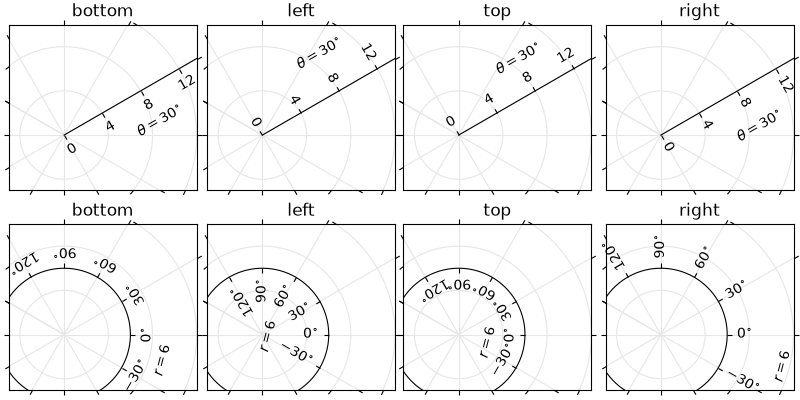
def add_floating_axis1(ax):
    ax.axis["lat"] = axis = ax.new_floating_axis(0, 30)
    axis.label.set_text(r"$\theta = 30^{\circ}$")
    axis.label.set_visible(True)
    return axis


def add_floating_axis2(ax):
    ax.axis["lon"] = axis = ax.new_floating_axis(1, 6)
    axis.label.set_text(r"$r = 6$")
    axis.label.set_visible(True)
    return axis


fig = plt.figure(figsize=(8, 4), layout="constrained")

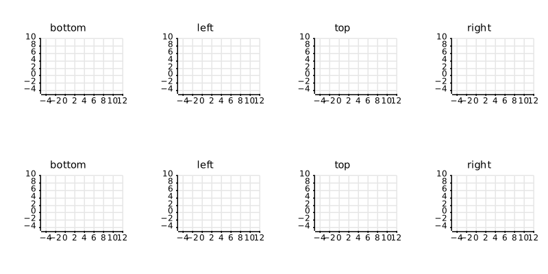
for i, d in enumerate(["bottom", "left", "top", "right"]):
    ax = setup_axes(fig, rect=241+i)
    axis = add_floating_axis1(ax)
    axis.set_axis_direction(d)
    ax.set(title=d)

for i, d in enumerate(["bottom", "left", "top", "right"]):
    ax = setup_axes(fig, rect=245+i)
    axis = add_floating_axis2(ax)
    axis.set_axis_direction(d)
    ax.set(title=d)

plt.show()
axisartist/demo_axisline_style
================
Source
"""
================
Axis line styles
================

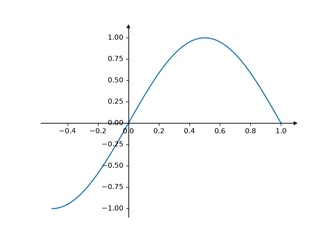
This example shows some configurations for axis style.

Note: The `mpl_toolkits.axisartist` Axes classes may be confusing for new
users. If the only aim is to obtain arrow heads at the ends of the axes,
rather check out the :doc:`/gallery/spines/centered_spines_with_arrows`
example.
"""

import matplotlib.pyplot as plt
import numpy as np

from mpl_toolkits.axisartist.axislines import AxesZero

fig = plt.figure()
ax = fig.add_subplot(axes_class=AxesZero)

for direction in ["xzero", "yzero"]:
    # adds arrows at the ends of each axis
    ax.axis[direction].set_axisline_style("-|>")

    # adds X and Y-axis from the origin
    ax.axis[direction].set_visible(True)

for direction in ["left", "right", "bottom", "top"]:
    # hides borders
    ax.axis[direction].set_visible(False)

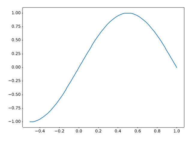
x = np.linspace(-0.5, 1., 100)
ax.plot(x, np.sin(x*np.pi))

plt.show()
axisartist/demo_curvelinear_grid
=====================
Source
"""
=====================
Curvilinear grid demo
=====================

Custom grid and ticklines.

This example demonstrates how to use
`~.grid_helper_curvelinear.GridHelperCurveLinear` to define custom grids and
ticklines by applying a transformation on the grid.  This can be used, as
shown on the second plot, to create polar projections in a rectangular box.
"""

import matplotlib.pyplot as plt
import numpy as np

from matplotlib.projections import PolarAxes
from matplotlib.transforms import Affine2D
from mpl_toolkits.axisartist import Axes, HostAxes, angle_helper
from mpl_toolkits.axisartist.grid_helper_curvelinear import GridHelperCurveLinear


def curvelinear_test1(fig):
    """
    Grid for custom transform.
    """

    def tr(x, y): return x, y - x
    def inv_tr(x, y): return x, y + x

    grid_helper = GridHelperCurveLinear((tr, inv_tr))

    ax1 = fig.add_subplot(1, 2, 1, axes_class=Axes, grid_helper=grid_helper)
    # ax1 will have ticks and gridlines defined by the given transform (+
    # transData of the Axes).  Note that the transform of the Axes itself
    # (i.e., transData) is not affected by the given transform.
    xx, yy = tr(np.array([3, 6]), np.array([5, 10]))
    ax1.plot(xx, yy)

    ax1.set_aspect(1)
    ax1.set_xlim(0, 10)
    ax1.set_ylim(0, 10)

    ax1.axis["t"] = ax1.new_floating_axis(0, 3)
    ax1.axis["t2"] = ax1.new_floating_axis(1, 7)
    ax1.grid(True, zorder=0)


def curvelinear_test2(fig):
    """
    Polar projection, but in a rectangular box.
    """

    # PolarAxes.PolarTransform takes radian. However, we want our coordinate
    # system in degree
    tr = Affine2D().scale(np.pi/180, 1) + PolarAxes.PolarTransform()
    # Polar projection, which involves cycle, and also has limits in
    # its coordinates, needs a special method to find the extremes
    # (min, max of the coordinate within the view).
    extreme_finder = angle_helper.ExtremeFinderCycle(
        nx=20, ny=20,  # Number of sampling points in each direction.
        lon_cycle=360, lat_cycle=None,
        lon_minmax=None, lat_minmax=(0, np.inf),
    )
    # Find grid values appropriate for the coordinate (degree, minute, second).
    grid_locator1 = angle_helper.LocatorDMS(12)
    # Use an appropriate formatter.  Note that the acceptable Locator and
    # Formatter classes are a bit different than that of Matplotlib, which
    # cannot directly be used here (this may be possible in the future).
    tick_formatter1 = angle_helper.FormatterDMS()

    grid_helper = GridHelperCurveLinear(
        tr, extreme_finder=extreme_finder,
        grid_locator1=grid_locator1, tick_formatter1=tick_formatter1)
    ax1 = fig.add_subplot(
        1, 2, 2, axes_class=HostAxes, grid_helper=grid_helper)

    # make ticklabels of right and top axis visible.
    ax1.axis["right"].major_ticklabels.set_visible(True)
    ax1.axis["top"].major_ticklabels.set_visible(True)
    # let right axis shows ticklabels for 1st coordinate (angle)
    ax1.axis["right"].get_helper().nth_coord_ticks = 0
    # let bottom axis shows ticklabels for 2nd coordinate (radius)
    ax1.axis["bottom"].get_helper().nth_coord_ticks = 1

    ax1.set_aspect(1)
    ax1.set_xlim(-5, 12)
    ax1.set_ylim(-5, 10)

    ax1.grid(True, zorder=0)

    # A parasite Axes with given transform
    ax2 = ax1.get_aux_axes(tr)
    # note that ax2.transData == tr + ax1.transData
    # Anything you draw in ax2 will match the ticks and grids of ax1.
    ax2.plot(np.linspace(0, 30, 51), np.linspace(10, 10, 51), linewidth=2)

    ax2.pcolor(np.linspace(0, 90, 4), np.linspace(0, 10, 4),
               np.arange(9).reshape((3, 3)))
    ax2.contour(np.linspace(0, 90, 4), np.linspace(0, 10, 4),
                np.arange(16).reshape((4, 4)), colors="k")


if __name__ == "__main__":
    fig = plt.figure(figsize=(7, 4))

    curvelinear_test1(fig)
    curvelinear_test2(fig)

    plt.show()
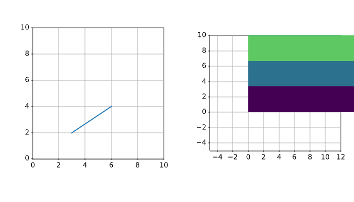
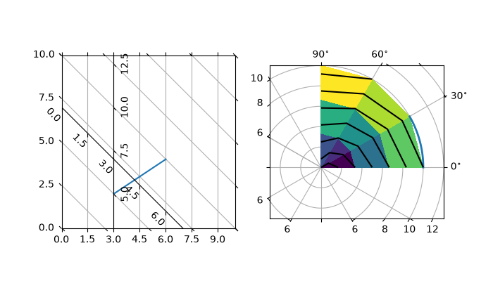
axisartist/demo_curvelinear_grid2
======================
Source
"""
======================
Demo CurveLinear Grid2
======================

Custom grid and ticklines.

This example demonstrates how to use GridHelperCurveLinear to define
custom grids and ticklines by applying a transformation on the grid.
As showcase on the plot, a 5x5 matrix is displayed on the Axes.
"""

import matplotlib.pyplot as plt
import numpy as np

from mpl_toolkits.axisartist.axislines import Axes
from mpl_toolkits.axisartist.grid_finder import ExtremeFinderSimple, MaxNLocator
from mpl_toolkits.axisartist.grid_helper_curvelinear import GridHelperCurveLinear


def curvelinear_test1(fig):
    """Grid for custom transform."""

    def tr(x, y):
        return np.sign(x)*abs(x)**.5, y

    def inv_tr(x, y):
        return np.sign(x)*x**2, y

    grid_helper = GridHelperCurveLinear(
        (tr, inv_tr),
        extreme_finder=ExtremeFinderSimple(20, 20),
        # better tick density
        grid_locator1=MaxNLocator(nbins=6), grid_locator2=MaxNLocator(nbins=6))

    ax1 = fig.add_subplot(axes_class=Axes, grid_helper=grid_helper)
    # ax1 will have a ticks and gridlines defined by the given
    # transform (+ transData of the Axes). Note that the transform of the Axes
    # itself (i.e., transData) is not affected by the given transform.

    ax1.imshow(np.arange(25).reshape(5, 5),
               vmax=50, cmap="gray_r", origin="lower")


if __name__ == "__main__":
    fig = plt.figure(figsize=(7, 4))
    curvelinear_test1(fig)
    plt.show()
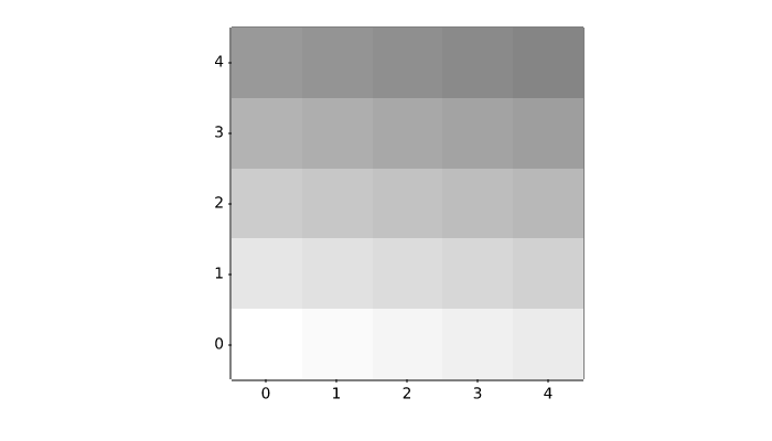
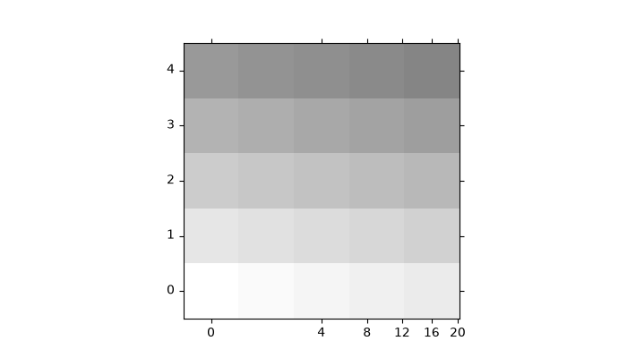
axisartist/demo_floating_axes
==========================
Source
"""
==========================
``floating_axes`` features
==========================

Demonstration of features of the :mod:`.floating_axes` module:

* Using `~.axes.Axes.scatter` and `~.axes.Axes.bar` with changing the shape of
  the plot.
* Using `~.floating_axes.GridHelperCurveLinear` to rotate the plot and set the
  plot boundary.
* Using `~.Figure.add_subplot` to create a subplot using the return value from
  `~.floating_axes.GridHelperCurveLinear`.
* Making a sector plot by adding more features to
  `~.floating_axes.GridHelperCurveLinear`.
"""

import matplotlib.pyplot as plt
import numpy as np

from matplotlib.projections import PolarAxes
from matplotlib.transforms import Affine2D
import mpl_toolkits.axisartist.angle_helper as angle_helper
import mpl_toolkits.axisartist.floating_axes as floating_axes
from mpl_toolkits.axisartist.grid_finder import DictFormatter, FixedLocator, MaxNLocator

# Fixing random state for reproducibility
np.random.seed(19680801)


def setup_axes1(fig, rect):
    """
    A simple one.
    """
    tr = Affine2D().scale(2, 1).rotate_deg(30)

    grid_helper = floating_axes.GridHelperCurveLinear(
        tr, extremes=(-0.5, 3.5, 0, 4),
        grid_locator1=MaxNLocator(nbins=4),
        grid_locator2=MaxNLocator(nbins=4))

    ax1 = fig.add_subplot(
        rect, axes_class=floating_axes.FloatingAxes, grid_helper=grid_helper)
    ax1.grid()

    aux_ax = ax1.get_aux_axes(tr)

    return ax1, aux_ax


def setup_axes2(fig, rect):
    """
    With custom locator and formatter.
    Note that the extreme values are swapped.
    """
    tr = PolarAxes.PolarTransform()

    pi = np.pi
    angle_ticks = {
        0: r"$0$",
        pi/4: r"$\frac{1}{4}\pi$",
        pi/2: r"$\frac{1}{2}\pi$",
    }
    grid_helper = floating_axes.GridHelperCurveLinear(
        tr, extremes=(.5*pi, 0, 2, 1),
        grid_locator1=FixedLocator([*angle_ticks]),
        tick_formatter1=DictFormatter(angle_ticks),
        grid_locator2=MaxNLocator(2),
        tick_formatter2=None,
    )
    ax1 = fig.add_subplot(
        rect, axes_class=floating_axes.FloatingAxes, grid_helper=grid_helper)
    ax1.grid()

    # create a parasite Axes whose transData in RA, cz
    aux_ax = ax1.get_aux_axes(tr)

    aux_ax.patch = ax1.patch  # for aux_ax to have a clip path as in ax
    ax1.patch.zorder = 0.9  # but this has a side effect that the patch is
    # drawn twice, and possibly over some other
    # artists. So, we decrease the zorder a bit to
    # prevent this.

    return ax1, aux_ax


def setup_axes3(fig, rect):
    """
    Sometimes, things like axis_direction need to be adjusted.
    """

    tr_rotate = Affine2D().translate(-95, 0)  # rotate a bit for better orientation
    tr_scale = Affine2D().scale(np.pi/180., 1.)  # scale degree to radians
    tr = tr_rotate + tr_scale + PolarAxes.PolarTransform()

    # Specify theta limits in degrees
    ra0, ra1 = 8.*15, 14.*15
    # Specify radial limits
    cz0, cz1 = 0, 14000

    grid_helper = floating_axes.GridHelperCurveLinear(
        tr, extremes=(ra0, ra1, cz0, cz1),
        grid_locator1=angle_helper.LocatorHMS(4),
        tick_formatter1=angle_helper.FormatterHMS(),
        grid_locator2=MaxNLocator(3),
        tick_formatter2=None,
    )
    ax1 = fig.add_subplot(
        rect, axes_class=floating_axes.FloatingAxes, grid_helper=grid_helper)

    # adjust axis
    ax1.axis["left"].set_axis_direction("bottom")
    ax1.axis["right"].set_axis_direction("top")

    ax1.axis["bottom"].set_visible(False)
    ax1.axis["top"].set_axis_direction("bottom")
    ax1.axis["top"].toggle(ticklabels=True, label=True)
    ax1.axis["top"].major_ticklabels.set_axis_direction("top")
    ax1.axis["top"].label.set_axis_direction("top")

    ax1.axis["left"].label.set_text(r"cz [km$^{-1}$]")
    ax1.axis["top"].label.set_text(r"$\alpha_{1950}$")
    ax1.grid()

    # create a parasite Axes whose transData in RA, cz
    aux_ax = ax1.get_aux_axes(tr)

    aux_ax.patch = ax1.patch  # for aux_ax to have a clip path as in ax
    ax1.patch.zorder = 0.9  # but this has a side effect that the patch is
    # drawn twice, and possibly over some other
    # artists. So, we decrease the zorder a bit to
    # prevent this.

    return ax1, aux_ax


# %%
fig = plt.figure(figsize=(8, 4))
fig.subplots_adjust(wspace=0.3, left=0.05, right=0.95)

ax1, aux_ax1 = setup_axes1(fig, 131)
aux_ax1.bar([0, 1, 2, 3], [3, 2, 1, 3])

ax2, aux_ax2 = setup_axes2(fig, 132)
theta = np.random.rand(10)*.5*np.pi
radius = np.random.rand(10) + 1.
aux_ax2.scatter(theta, radius)

ax3, aux_ax3 = setup_axes3(fig, 133)

theta = (8 + np.random.rand(10)*(14 - 8))*15.  # in degrees
radius = np.random.rand(10)*14000.
aux_ax3.scatter(theta, radius)

plt.show()
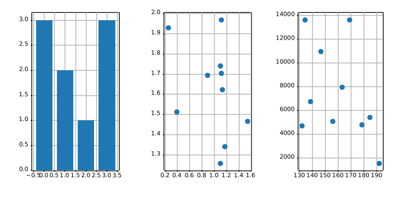
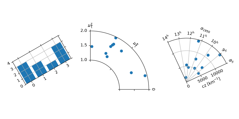
axisartist/demo_floating_axis
==================
Source
"""
==================
floating_axis demo
==================

Axis within rectangular frame.

The following code demonstrates how to put a floating polar curve within a
rectangular box. In order to get a better sense of polar curves, please look at
:doc:`/gallery/axisartist/demo_curvelinear_grid`.
"""

import matplotlib.pyplot as plt
import numpy as np

from matplotlib.projections import PolarAxes
from matplotlib.transforms import Affine2D
from mpl_toolkits.axisartist import GridHelperCurveLinear, HostAxes
import mpl_toolkits.axisartist.angle_helper as angle_helper


def curvelinear_test2(fig):
    """Polar projection, but in a rectangular box."""
    # see demo_curvelinear_grid.py for details
    grid_helper = GridHelperCurveLinear(
        Affine2D().scale(np.pi / 180., 1.) + PolarAxes.PolarTransform(),
        extreme_finder=angle_helper.ExtremeFinderCycle(
            20, 20,
            lon_cycle=360, lat_cycle=None,
            lon_minmax=None, lat_minmax=(0, np.inf),
        ),
        grid_locator1=angle_helper.LocatorDMS(12),
        tick_formatter1=angle_helper.FormatterDMS(),
    )
    ax1 = fig.add_subplot(axes_class=HostAxes, grid_helper=grid_helper)

    # Now create floating axis

    # floating axis whose first coordinate (theta) is fixed at 60
    ax1.axis["lat"] = axis = ax1.new_floating_axis(0, 60)
    axis.label.set_text(r"$\theta = 60^{\circ}$")
    axis.label.set_visible(True)

    # floating axis whose second coordinate (r) is fixed at 6
    ax1.axis["lon"] = axis = ax1.new_floating_axis(1, 6)
    axis.label.set_text(r"$r = 6$")

    ax1.set_aspect(1.)
    ax1.set_xlim(-5, 12)
    ax1.set_ylim(-5, 10)

    ax1.grid(True)


fig = plt.figure(figsize=(5, 5))
curvelinear_test2(fig)
plt.show()
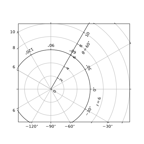
axisartist/demo_parasite_axes
==================
Source
"""
==================
Parasite Axes demo
==================

Create a parasite Axes. Such Axes would share the x scale with a host Axes,
but show a different scale in y direction.

This approach uses `mpl_toolkits.axes_grid1.parasite_axes.HostAxes` and
`mpl_toolkits.axes_grid1.parasite_axes.ParasiteAxes`.

The standard and recommended approach is to use instead standard Matplotlib
axes, as shown in the
:doc:`/gallery/subplots_axes_and_figures/multiple_yaxis_with_spines` example.

An alternative approach using `mpl_toolkits.axes_grid1` and
`mpl_toolkits.axisartist` is shown in the
:doc:`/gallery/axisartist/demo_parasite_axes2` example.
"""

import matplotlib.pyplot as plt

from mpl_toolkits.axisartist.parasite_axes import HostAxes

fig = plt.figure()

host = fig.add_axes((0.15, 0.1, 0.65, 0.8), axes_class=HostAxes)
par1 = host.get_aux_axes(viewlim_mode=None, sharex=host)
par2 = host.get_aux_axes(viewlim_mode=None, sharex=host)

host.axis["right"].set_visible(False)

par1.axis["right"].set_visible(True)
par1.axis["right"].major_ticklabels.set_visible(True)
par1.axis["right"].label.set_visible(True)

par2.axis["right2"] = par2.new_fixed_axis(loc="right", offset=(60, 0))

p1, = host.plot([0, 1, 2], [0, 1, 2], label="Density")
p2, = par1.plot([0, 1, 2], [0, 3, 2], label="Temperature")
p3, = par2.plot([0, 1, 2], [50, 30, 15], label="Velocity")

host.set(xlim=(0, 2), ylim=(0, 2), xlabel="Distance", ylabel="Density")
par1.set(ylim=(0, 4), ylabel="Temperature")
par2.set(ylim=(1, 65), ylabel="Velocity")

host.legend()

host.axis["left"].label.set_color(p1.get_color())
par1.axis["right"].label.set_color(p2.get_color())
par2.axis["right2"].label.set_color(p3.get_color())

plt.show()
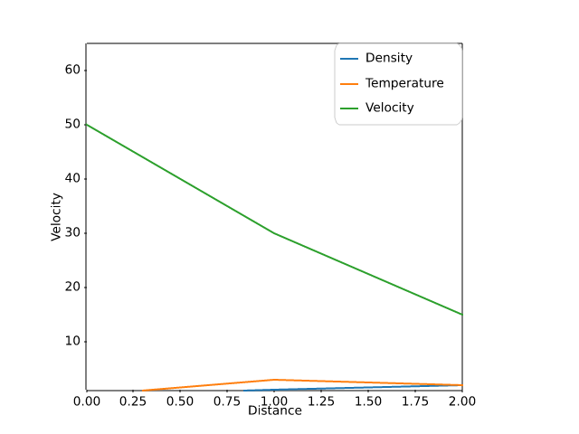
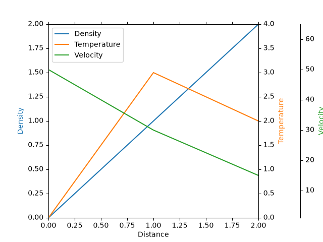
axisartist/demo_parasite_axes2
==================
Source
"""
==================
Parasite axis demo
==================

This example demonstrates the use of parasite axis to plot multiple datasets
onto one single plot.

Notice how in this example, *par1* and *par2* are both obtained by calling
``twinx()``, which ties their x-limits with the host's x-axis. From there, each
of those two axis behave separately from each other: different datasets can be
plotted, and the y-limits are adjusted separately.

This approach uses `mpl_toolkits.axes_grid1.parasite_axes.host_subplot` and
`mpl_toolkits.axisartist.axislines.Axes`.

The standard and recommended approach is to use instead standard Matplotlib
axes, as shown in the
:doc:`/gallery/subplots_axes_and_figures/multiple_yaxis_with_spines` example.

An alternative approach using `mpl_toolkits.axes_grid1.parasite_axes.HostAxes`
and `mpl_toolkits.axes_grid1.parasite_axes.ParasiteAxes` is shown in the
:doc:`/gallery/axisartist/demo_parasite_axes` example.
"""

import matplotlib.pyplot as plt

from mpl_toolkits import axisartist
from mpl_toolkits.axes_grid1 import host_subplot

host = host_subplot(111, axes_class=axisartist.Axes)
plt.subplots_adjust(right=0.75)

par1 = host.twinx()
par2 = host.twinx()

par2.axis["right"] = par2.new_fixed_axis(loc="right", offset=(60, 0))

par1.axis["right"].toggle(all=True)
par2.axis["right"].toggle(all=True)

p1, = host.plot([0, 1, 2], [0, 1, 2], label="Density")
p2, = par1.plot([0, 1, 2], [0, 3, 2], label="Temperature")
p3, = par2.plot([0, 1, 2], [50, 30, 15], label="Velocity")

host.set(xlim=(0, 2), ylim=(0, 2), xlabel="Distance", ylabel="Density")
par1.set(ylim=(0, 4), ylabel="Temperature")
par2.set(ylim=(1, 65), ylabel="Velocity")

host.legend()

host.axis["left"].label.set_color(p1.get_color())
par1.axis["right"].label.set_color(p2.get_color())
par2.axis["right"].label.set_color(p3.get_color())

plt.show()
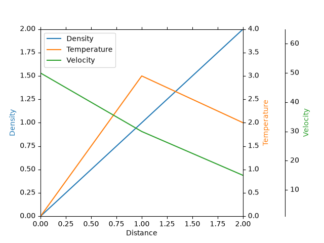
axisartist/demo_ticklabel_alignment
===================
Source
"""
===================
Ticklabel alignment
===================

"""


import matplotlib.pyplot as plt

import mpl_toolkits.axisartist as axisartist


def setup_axes(fig, pos):
    ax = fig.add_subplot(pos, axes_class=axisartist.Axes)
    ax.set_yticks([0.2, 0.8], labels=["short", "loooong"])
    ax.set_xticks([0.2, 0.8], labels=[r"$\frac{1}{2}\pi$", r"$\pi$"])
    return ax


fig = plt.figure(figsize=(3, 5))
fig.subplots_adjust(left=0.5, hspace=0.7)

ax = setup_axes(fig, 311)
ax.set_ylabel("ha=right")
ax.set_xlabel("va=baseline")

ax = setup_axes(fig, 312)
ax.axis["left"].major_ticklabels.set_ha("center")
ax.axis["bottom"].major_ticklabels.set_va("top")
ax.set_ylabel("ha=center")
ax.set_xlabel("va=top")

ax = setup_axes(fig, 313)
ax.axis["left"].major_ticklabels.set_ha("left")
ax.axis["bottom"].major_ticklabels.set_va("bottom")
ax.set_ylabel("ha=left")
ax.set_xlabel("va=bottom")

plt.show()
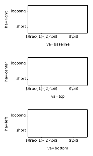
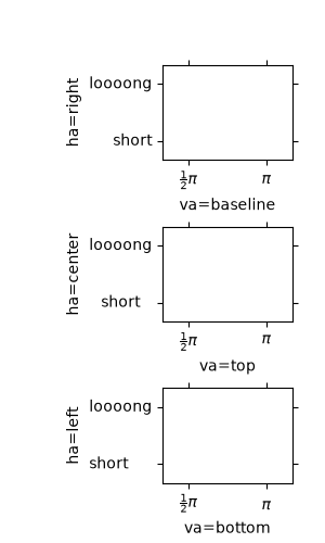
axisartist/demo_ticklabel_direction
===================
Source
"""
===================
Ticklabel direction
===================

"""

import matplotlib.pyplot as plt

import mpl_toolkits.axisartist.axislines as axislines


def setup_axes(fig, pos):
    ax = fig.add_subplot(pos, axes_class=axislines.Axes)
    ax.set_yticks([0.2, 0.8])
    ax.set_xticks([0.2, 0.8])
    return ax


fig = plt.figure(figsize=(6, 3))
fig.subplots_adjust(bottom=0.2)

ax = setup_axes(fig, 131)
for axis in ax.axis.values():
    axis.major_ticks.set_tick_out(True)
# or you can simply do "ax.axis[:].major_ticks.set_tick_out(True)"

ax = setup_axes(fig, 132)
ax.axis["left"].set_axis_direction("right")
ax.axis["bottom"].set_axis_direction("top")
ax.axis["right"].set_axis_direction("left")
ax.axis["top"].set_axis_direction("bottom")

ax = setup_axes(fig, 133)
ax.axis["left"].set_axis_direction("right")
ax.axis[:].major_ticks.set_tick_out(True)

ax.axis["left"].label.set_text("Long Label Left")
ax.axis["bottom"].label.set_text("Label Bottom")
ax.axis["right"].label.set_text("Long Label Right")
ax.axis["right"].label.set_visible(True)
ax.axis["left"].label.set_pad(0)
ax.axis["bottom"].label.set_pad(10)

plt.show()
axisartist/simple_axis_direction01
=====================
Source
"""
=====================
Simple axis direction
=====================

"""
import matplotlib.pyplot as plt

import mpl_toolkits.axisartist as axisartist

fig = plt.figure(figsize=(4, 2.5))
ax1 = fig.add_subplot(axes_class=axisartist.Axes)
fig.subplots_adjust(right=0.8)

ax1.axis["left"].major_ticklabels.set_axis_direction("top")
ax1.axis["left"].label.set_text("Left label")

ax1.axis["right"].label.set_visible(True)
ax1.axis["right"].label.set_text("Right label")
ax1.axis["right"].label.set_axis_direction("left")

plt.show()
axisartist/simple_axis_direction03
==========================================
Source
"""
==========================================
Simple axis tick label and tick directions
==========================================

First subplot moves the tick labels to inside the spines.
Second subplot moves the ticks to inside the spines.
These effects can be obtained for a standard Axes by `~.Axes.tick_params`.
"""

import matplotlib.pyplot as plt

import mpl_toolkits.axisartist as axisartist


def setup_axes(fig, pos):
    ax = fig.add_subplot(pos, axes_class=axisartist.Axes)
    ax.set_yticks([0.2, 0.8])
    ax.set_xticks([0.2, 0.8])
    return ax


fig = plt.figure(figsize=(5, 2))
fig.subplots_adjust(wspace=0.4, bottom=0.3)

ax1 = setup_axes(fig, 121)
ax1.set_xlabel("ax1 X-label")
ax1.set_ylabel("ax1 Y-label")

ax1.axis[:].invert_ticklabel_direction()

ax2 = setup_axes(fig, 122)
ax2.set_xlabel("ax2 X-label")
ax2.set_ylabel("ax2 Y-label")

ax2.axis[:].major_ticks.set_tick_out(False)

plt.show()
axisartist/simple_axis_pad
===============
Source
"""
===============
Simple axis pad
===============

"""

import matplotlib.pyplot as plt
import numpy as np

from matplotlib.projections import PolarAxes
from matplotlib.transforms import Affine2D
import mpl_toolkits.axisartist as axisartist
from mpl_toolkits.axisartist import angle_helper, grid_finder
from mpl_toolkits.axisartist.grid_helper_curvelinear import GridHelperCurveLinear


def setup_axes(fig, rect):
    """Polar projection, but in a rectangular box."""
    # see demo_curvelinear_grid.py for details
    grid_helper = GridHelperCurveLinear(
        Affine2D().scale(np.pi/180., 1.) + PolarAxes.PolarTransform(),
        extreme_finder=angle_helper.ExtremeFinderCycle(
            20, 20,
            lon_cycle=360, lat_cycle=None,
            lon_minmax=None, lat_minmax=(0, np.inf),
        ),
        grid_locator1=angle_helper.LocatorDMS(12),
        grid_locator2=grid_finder.MaxNLocator(5),
        tick_formatter1=angle_helper.FormatterDMS(),
    )
    ax = fig.add_subplot(
        rect, axes_class=axisartist.Axes, grid_helper=grid_helper,
        aspect=1, xlim=(-5, 12), ylim=(-5, 10))
    ax.axis[:].set_visible(False)
    return ax


def add_floating_axis1(ax1):
    ax1.axis["lat"] = axis = ax1.new_floating_axis(0, 30)
    axis.label.set_text(r"$\theta = 30^{\circ}$")
    axis.label.set_visible(True)

    return axis


def add_floating_axis2(ax1):
    ax1.axis["lon"] = axis = ax1.new_floating_axis(1, 6)
    axis.label.set_text(r"$r = 6$")
    axis.label.set_visible(True)

    return axis


fig = plt.figure(figsize=(9, 3.))
fig.subplots_adjust(left=0.01, right=0.99, bottom=0.01, top=0.99,
                    wspace=0.01, hspace=0.01)


def ann(ax1, d):
    ax1.annotate(d, (0.5, 1), (5, -5),
                 xycoords="axes fraction", textcoords="offset points",
                 va="top", ha="center")


ax1 = setup_axes(fig, rect=231)
axis = add_floating_axis1(ax1)
ann(ax1, "default")

ax1 = setup_axes(fig, rect=232)
axis = add_floating_axis1(ax1)
axis.major_ticklabels.set_pad(10)
ann(ax1, "ticklabels.set_pad(10)")

ax1 = setup_axes(fig, rect=233)
axis = add_floating_axis1(ax1)
axis.label.set_pad(20)
ann(ax1, "label.set_pad(20)")

ax1 = setup_axes(fig, rect=234)
axis = add_floating_axis1(ax1)
axis.major_ticks.set_tick_direction("in")
ann(ax1, 'ticks.set_tick_direction("in")')

ax1 = setup_axes(fig, rect=235)
axis = add_floating_axis1(ax1)
axis.major_ticks.set_tick_direction("out")
ann(ax1, 'ticks.set_tick_direction("out")')

ax1 = setup_axes(fig, rect=236)
axis = add_floating_axis1(ax1)
axis.major_ticks.set_tick_direction("inout")
ann(ax1, 'ticks.set_tick_direction("inout")')

plt.show()
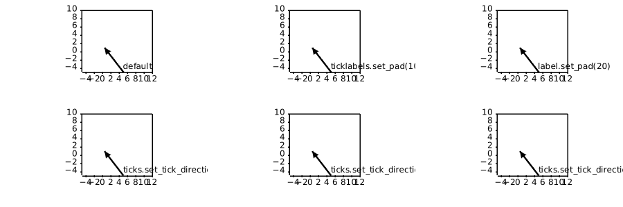
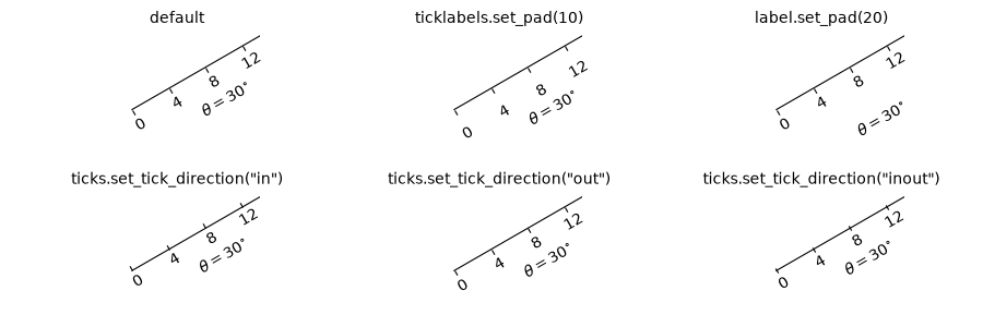
axisartist/simple_axisartist1
=============================
Source
"""
=============================
Custom spines with axisartist
=============================

This example showcases the use of :mod:`.axisartist` to draw spines at custom
positions (here, at ``y = 0``).

Note, however, that it is simpler to achieve this effect using standard
`.Spine` methods, as demonstrated in
:doc:`/gallery/spines/centered_spines_with_arrows`.

.. redirect-from:: /gallery/axisartist/simple_axisline2
"""

import matplotlib.pyplot as plt
import numpy as np

from mpl_toolkits import axisartist

fig = plt.figure(figsize=(6, 3), layout="constrained")
# To construct Axes of two different classes, we need to use gridspec (or
# MATLAB-style add_subplot calls).
gs = fig.add_gridspec(1, 2)


ax0 = fig.add_subplot(gs[0, 0], axes_class=axisartist.Axes)
# Make a new axis along the first (x) axis which passes through y=0.
ax0.axis["y=0"] = ax0.new_floating_axis(nth_coord=0, value=0,
                                        axis_direction="bottom")
ax0.axis["y=0"].toggle(all=True)
ax0.axis["y=0"].label.set_text("y = 0")
# Make other axis invisible.
ax0.axis["bottom", "top", "right"].set_visible(False)


# Alternatively, one can use AxesZero, which automatically sets up two
# additional axis, named "xzero" (the y=0 axis) and "yzero" (the x=0 axis).
ax1 = fig.add_subplot(gs[0, 1], axes_class=axisartist.axislines.AxesZero)
# "xzero" and "yzero" default to invisible; make xzero axis visible.
ax1.axis["xzero"].set_visible(True)
ax1.axis["xzero"].label.set_text("Axis Zero")
# Make other axis invisible.
ax1.axis["bottom", "top", "right"].set_visible(False)


# Draw some sample data.
x = np.arange(0, 2*np.pi, 0.01)
ax0.plot(x, np.sin(x))
ax1.plot(x, np.sin(x))

plt.show()
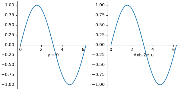
axisartist/simple_axisline
===============
Source
"""
===============
Simple Axisline
===============

"""

import matplotlib.pyplot as plt

from mpl_toolkits.axisartist.axislines import AxesZero

fig = plt.figure()
fig.subplots_adjust(right=0.85)
ax = fig.add_subplot(axes_class=AxesZero)

# make right and top axis invisible
ax.axis["right"].set_visible(False)
ax.axis["top"].set_visible(False)

# make xzero axis (horizontal axis line through y=0) visible.
ax.axis["xzero"].set_visible(True)
ax.axis["xzero"].label.set_text("Axis Zero")

ax.set_ylim(-2, 4)
ax.set_xlabel("Label X")
ax.set_ylabel("Label Y")
# Or:
# ax.axis["bottom"].label.set_text("Label X")
# ax.axis["left"].label.set_text("Label Y")

# make new (right-side) yaxis, but with some offset
ax.axis["right2"] = ax.new_fixed_axis(loc="right", offset=(20, 0))
ax.axis["right2"].label.set_text("Label Y2")

ax.plot([-2, 3, 2])
plt.show()
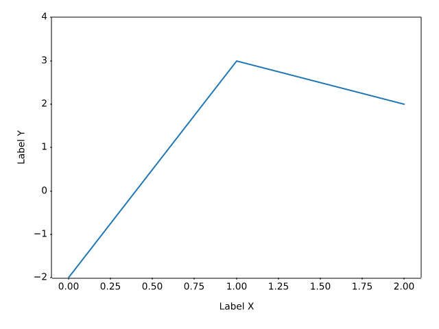
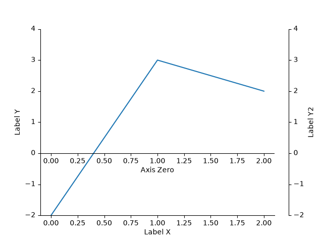
axisartist/simple_axisline3
================
Source
"""
================
Simple Axisline3
================

"""
import matplotlib.pyplot as plt

from mpl_toolkits.axisartist.axislines import Axes

fig = plt.figure(figsize=(3, 3))

ax = fig.add_subplot(axes_class=Axes)

ax.axis["right"].set_visible(False)
ax.axis["top"].set_visible(False)

plt.show()
color/color_by_yvalue
================
Source
"""
================
Color by y-value
================

Use masked arrays to plot a line with different colors by y-value.
"""
import matplotlib.pyplot as plt
import numpy as np

t = np.arange(0.0, 2.0, 0.01)
s = np.sin(2 * np.pi * t)

upper = 0.77
lower = -0.77

supper = np.ma.masked_where(s < upper, s)
slower = np.ma.masked_where(s > lower, s)
smiddle = np.ma.masked_where((s < lower) | (s > upper), s)

fig, ax = plt.subplots()
ax.plot(t, smiddle, t, slower, t, supper)
plt.show()

# %%
#
# .. admonition:: References
#
#    The use of the following functions, methods, classes and modules is shown
#    in this example:
#
#    - `matplotlib.axes.Axes.plot` / `matplotlib.pyplot.plot`
#
# .. tags::
#
#    styling: color
#    styling: conditional
#    plot-type: line
#    level: beginner
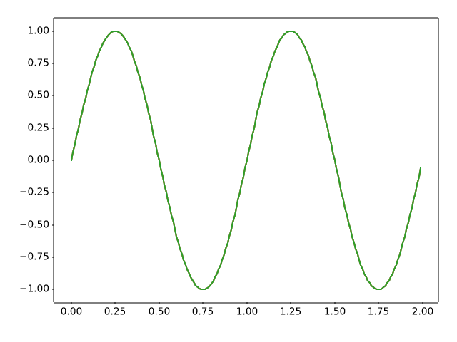
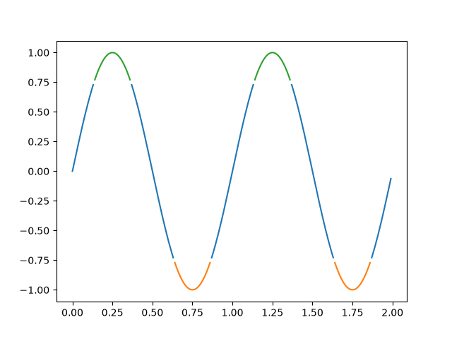
color/color_cycle_default
====================================
Source
"""
====================================
Colors in the default property cycle
====================================

Display the colors from the default prop_cycle, which is obtained from the
:ref:`rc parameters<customizing>`.
"""
import matplotlib.pyplot as plt
import numpy as np

from matplotlib.colors import TABLEAU_COLORS, same_color


def f(x, a):
    """A nice sigmoid-like parametrized curve, ending approximately at *a*."""
    return 0.85 * a * (1 / (1 + np.exp(-x)) + 0.2)


fig, ax = plt.subplots()
ax.axis('off')
ax.set_title("Colors in the default property cycle")

prop_cycle = plt.rcParams['axes.prop_cycle']
colors = prop_cycle.by_key()['color']
x = np.linspace(-4, 4, 200)

for i, (color, color_name) in enumerate(zip(colors, TABLEAU_COLORS)):
    assert same_color(color, color_name)
    pos = 4.5 - i
    ax.plot(x, f(x, pos))
    ax.text(4.2, pos, f"'C{i}': '{color_name}'", color=color, va="center")
    ax.bar(9, 1, width=1.5, bottom=pos-0.5)

plt.show()

# %%
#
# .. admonition:: References
#
#    The use of the following functions, methods, classes and modules is shown
#    in this example:
#
#    - `matplotlib.axes.Axes.axis`
#    - `matplotlib.axes.Axes.text`
#    - `matplotlib.colors.same_color`
#    - `cycler.Cycler`
#
# .. tags::
#
#    styling: color
#    purpose: reference
#    plot-type: line
#    level: beginner
color/color_demo
==========
Source
"""
==========
Color Demo
==========

Matplotlib recognizes the following formats to specify a color:

1) an RGB or RGBA tuple of float values in ``[0, 1]`` (e.g. ``(0.1, 0.2, 0.5)``
   or ``(0.1, 0.2, 0.5, 0.3)``).  RGBA is short for Red, Green, Blue, Alpha;
2) a hex RGB or RGBA string (e.g., ``'#0F0F0F'`` or ``'#0F0F0F0F'``);
3) a shorthand hex RGB or RGBA string, equivalent to the hex RGB or RGBA
   string obtained by duplicating each character, (e.g., ``'#abc'``, equivalent
   to ``'#aabbcc'``, or ``'#abcd'``, equivalent to ``'#aabbccdd'``);
4) a string representation of a float value in ``[0, 1]`` inclusive for gray
   level (e.g., ``'0.5'``);
5) a single letter string, i.e. one of
   ``{'b', 'g', 'r', 'c', 'm', 'y', 'k', 'w'}``, which are short-hand notations
   for shades of blue, green, red, cyan, magenta, yellow, black, and white;
6) an X11/CSS4 ("html") color name, e.g. ``"blue"``;
7) a name from the `xkcd color survey <https://xkcd.com/color/rgb/>`__,
   prefixed with ``'xkcd:'`` (e.g., ``'xkcd:sky blue'``);
8) a "Cn" color spec, i.e. ``'C'`` followed by a number, which is an index into
   the default property cycle (:rc:`axes.prop_cycle`); the indexing is intended
   to occur at rendering time, and defaults to black if the cycle does not
   include color.
9) one of ``{'tab:blue', 'tab:orange', 'tab:green', 'tab:red', 'tab:purple',
   'tab:brown', 'tab:pink', 'tab:gray', 'tab:olive', 'tab:cyan'}`` which are
   the Tableau Colors from the 'tab10' categorical palette (which is the
   default color cycle);

For more information on colors in matplotlib see

* the :ref:`colors_def` tutorial;
* the `matplotlib.colors` API;
* the :doc:`/gallery/color/named_colors` example.
"""

import matplotlib.pyplot as plt
import numpy as np

t = np.linspace(0.0, 2.0, 201)
s = np.sin(2 * np.pi * t)

# 1) RGB tuple:
fig, ax = plt.subplots(facecolor=(.18, .31, .31))
# 2) hex string:
ax.set_facecolor('#eafff5')
# 3) gray level string:
ax.set_title('Voltage vs. time chart', color='0.7')
# 4) single letter color string
ax.set_xlabel('Time [s]', color='c')
# 5) a named color:
ax.set_ylabel('Voltage [mV]', color='peachpuff')
# 6) a named xkcd color:
ax.plot(t, s, 'xkcd:crimson')
# 7) Cn notation:
ax.plot(t, .7*s, color='C4', linestyle='--')
# 8) tab notation:
ax.tick_params(labelcolor='tab:orange')


plt.show()

# %%
#
# .. admonition:: References
#
#    The use of the following functions, methods, classes and modules is shown
#    in this example:
#
#    - `matplotlib.colors`
#    - `matplotlib.axes.Axes.plot`
#    - `matplotlib.axes.Axes.set_facecolor`
#    - `matplotlib.axes.Axes.set_title`
#    - `matplotlib.axes.Axes.set_xlabel`
#    - `matplotlib.axes.Axes.set_ylabel`
#    - `matplotlib.axes.Axes.tick_params`
#
# .. tags::
#
#    styling: color
#    plot-type: line
#    level: beginner
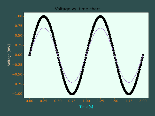
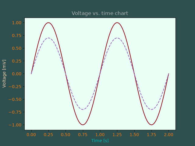
color/color_sequences
=====================
Source
"""
=====================
Named color sequences
=====================

Matplotlib's `~matplotlib.colors.ColorSequenceRegistry` allows access to
predefined lists of colors by name e.g.
``colors = matplotlib.color_sequences['Set1']``.  This example shows all of the
built in color sequences.

User-defined sequences can be added via `.ColorSequenceRegistry.register`.
"""

import matplotlib.pyplot as plt
import numpy as np

import matplotlib as mpl


def plot_color_sequences(names, ax):
    # Display each named color sequence horizontally on the supplied axes.

    for n, name in enumerate(names):
        colors = mpl.color_sequences[name]
        n_colors = len(colors)
        x = np.arange(n_colors)
        y = np.full_like(x, n)

        ax.scatter(x, y, facecolor=colors, edgecolor='dimgray', s=200, zorder=2)

    ax.set_yticks(range(len(names)), labels=names)
    ax.grid(visible=True, axis='y')
    ax.yaxis.set_inverted(True)
    ax.xaxis.set_visible(False)
    ax.spines[:].set_visible(False)
    ax.tick_params(left=False)


built_in_color_sequences = [
    'tab10', 'tab20', 'tab20b', 'tab20c', 'Pastel1', 'Pastel2', 'Paired',
    'Accent', 'okabe_ito', 'Dark2', 'Set1', 'Set2', 'Set3', 'petroff6',
    'petroff8', 'petroff10']


fig, ax = plt.subplots(figsize=(6.4, 9.6), layout='constrained')

plot_color_sequences(built_in_color_sequences, ax)
ax.set_title('Built In Color Sequences')

plt.show()


# %%
#
# .. admonition:: References
#
#    The use of the following functions, methods, classes and modules is shown
#    in this example:
#
#    - `matplotlib.colors.ColorSequenceRegistry`
#    - `matplotlib.axes.Axes.scatter`
#
# .. tags::
#
#    styling: color
#    purpose: reference
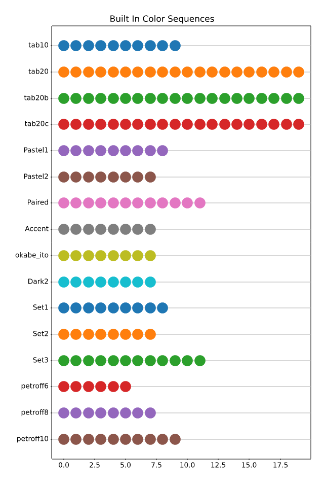
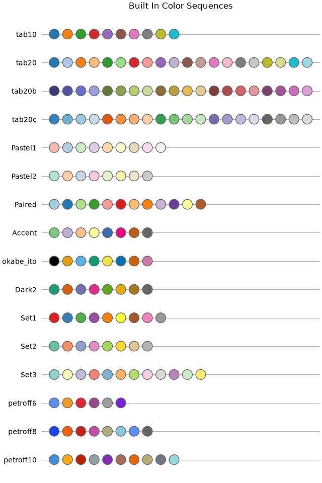
color/colorbar_basics
========
Source
"""
========
Colorbar
========

Use `~.Figure.colorbar` by specifying the mappable object (here
the `.AxesImage` returned by `~.axes.Axes.imshow`)
and the Axes to attach the colorbar to.
"""

import matplotlib.pyplot as plt
import numpy as np

# setup some generic data
N = 37
x, y = np.mgrid[:N, :N]
Z = (np.cos(x*0.2) + np.sin(y*0.3))

# mask out the negative and positive values, respectively
Zpos = np.ma.masked_less(Z, 0)
Zneg = np.ma.masked_greater(Z, 0)

fig, (ax1, ax2, ax3) = plt.subplots(figsize=(13, 3), ncols=3)

# plot just the positive data and save the
# color "mappable" object returned by ax1.imshow
pos = ax1.imshow(Zpos, cmap='Blues', interpolation='none')

# add the colorbar using the figure's method,
# telling which mappable we're talking about and
# which Axes object it should be near
fig.colorbar(pos, ax=ax1)

# repeat everything above for the negative data
# you can specify location, anchor and shrink the colorbar
neg = ax2.imshow(Zneg, cmap='Reds_r', interpolation='none')
fig.colorbar(neg, ax=ax2, location='right', anchor=(0, 0.3), shrink=0.7)

# Plot both positive and negative values between +/- 1.2
pos_neg_clipped = ax3.imshow(Z, cmap='RdBu', vmin=-1.2, vmax=1.2,
                             interpolation='none')
# Add minorticks on the colorbar to make it easy to read the
# values off the colorbar.
cbar = fig.colorbar(pos_neg_clipped, ax=ax3, extend='both')
cbar.minorticks_on()
plt.show()

# %%
#
# .. admonition:: References
#
#    The use of the following functions, methods, classes and modules is shown
#    in this example:
#
#    - `matplotlib.axes.Axes.imshow` / `matplotlib.pyplot.imshow`
#    - `matplotlib.figure.Figure.colorbar` / `matplotlib.pyplot.colorbar`
#    - `matplotlib.colorbar.Colorbar.minorticks_on`
#    - `matplotlib.colorbar.Colorbar.minorticks_off`
#
# .. tags::
#
#    component: colorbar
#    styling: color
#    plot-type: imshow
#    level: beginner
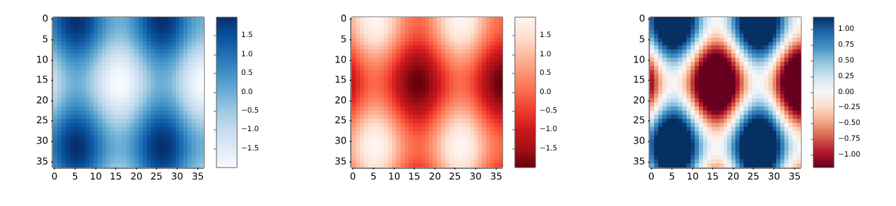
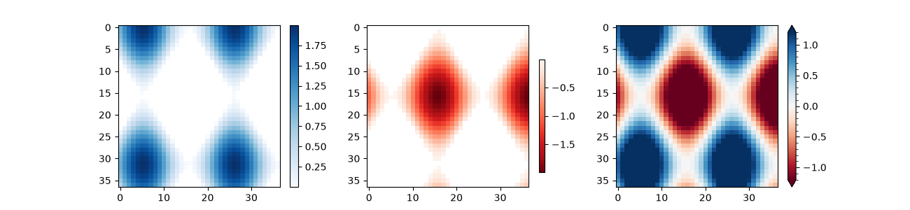
color/colorbar_histogram
=====================
Source
"""
=====================
Histogram as colorbar
=====================

This example demonstrates how to use a colored histogram instead of a colorbar
to not only show the color-to-value mapping, but also visualize the
distribution of values.
"""

import matplotlib.pyplot as plt
import numpy as np

import matplotlib.colors as mcolors

# surface data
delta = 0.025
x = y = np.arange(-2.0, 2.0, delta)
X, Y = np.meshgrid(x, y)
Z1 = np.exp(-(((X + 1) * 1.3) ** 2) - ((Y + 1) * 1.3) ** 2)
Z2 = 2.5 * np.exp(-((X - 1) ** 2) - (Y - 1) ** 2)
Z = Z1**0.25 - Z2**0.5

# colormap & normalization
bins = 30
cmap = plt.get_cmap("RdYlBu_r")
bin_edges = np.linspace(Z.min(), Z.max(), bins + 1)
norm = mcolors.BoundaryNorm(bin_edges, cmap.N)

# main plot
fig, ax = plt.subplots(layout="constrained")
im = ax.imshow(Z, cmap=cmap, origin="lower", extent=[-3, 3, -3, 3], norm=norm)

# inset histogram
cax = ax.inset_axes([1.18, 0.02, 0.25, 0.95])  # left, bottom, width, height

# plot histogram
counts, _ = np.histogram(Z, bins=bin_edges)
midpoints = (bin_edges[:-1] + bin_edges[1:]) / 2
distance = midpoints[1] - midpoints[0]
cax.barh(midpoints, counts, height=0.8 * distance, color=cmap(norm(midpoints)))

# styling
cax.spines[:].set_visible(False)
cax.set_yticks(bin_edges)
cax.tick_params(axis="both", which="both", length=0)

plt.show()
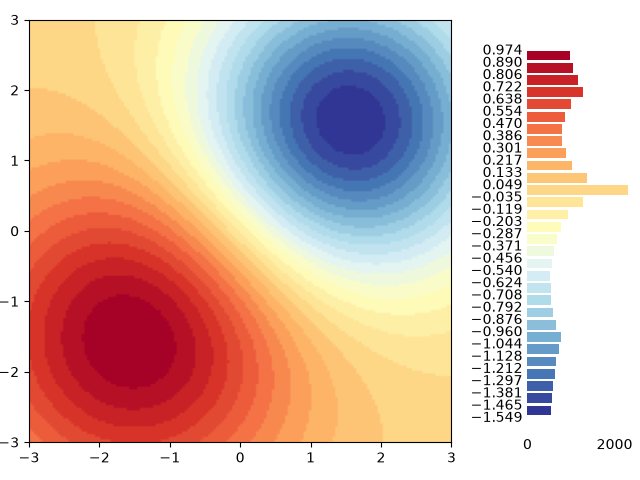
color/colormap_reference
==================
Source
"""
==================
Colormap reference
==================

Reference for colormaps included with Matplotlib.

A reversed version of each of these colormaps is available by appending
``_r`` to the name, as shown in :ref:`reverse-cmap`.

See :ref:`colormaps` for an in-depth discussion about
colormaps, including colorblind-friendliness, and
:ref:`colormap-manipulation` for a guide to creating
colormaps.
"""

import matplotlib.pyplot as plt
import numpy as np

cmaps = [('Perceptually Uniform Sequential', [
            'viridis', 'plasma', 'inferno', 'magma', 'cividis']),
         ('Sequential', [
            'Greys', 'Purples', 'Blues', 'Greens', 'Oranges', 'Reds',
            'YlOrBr', 'YlOrRd', 'OrRd', 'PuRd', 'RdPu', 'BuPu',
            'GnBu', 'PuBu', 'YlGnBu', 'PuBuGn', 'BuGn', 'YlGn']),
         ('Sequential (2)', [
            'gray', 'bone', 'pink', 'spring', 'summer', 'autumn', 'winter',
            'cool', 'Wistia', 'hot', 'afmhot', 'gist_heat', 'copper']),
         ('Diverging', [
            'PiYG', 'PRGn', 'BrBG', 'PuOr', 'RdGy', 'RdBu',
            'RdYlBu', 'RdYlGn', 'Spectral', 'coolwarm', 'bwr', 'seismic',
            'berlin', 'managua', 'vanimo']),
         ('Cyclic', ['twilight', 'twilight_shifted', 'hsv']),
         ('Qualitative', [
            'Pastel1', 'Pastel2', 'Paired', 'Accent', 'okabe_ito',
            'Dark2', 'Set1', 'Set2', 'Set3',
            'tab10', 'tab20', 'tab20b', 'tab20c']),
         ('Miscellaneous', [
            'flag', 'prism', 'ocean', 'gist_earth', 'terrain', 'gist_stern',
            'gnuplot', 'gnuplot2', 'CMRmap', 'cubehelix', 'brg',
            'gist_rainbow', 'rainbow', 'jet', 'turbo', 'nipy_spectral',
            'gist_ncar'])]

gradient = np.linspace(0, 1, 256)
gradient = np.vstack((gradient, gradient))


def plot_color_gradients(cmap_category, cmap_list):
    # Create figure and adjust figure height to number of colormaps
    nrows = len(cmap_list)
    figh = 0.35 + 0.15 + (nrows + (nrows-1)*0.1)*0.22
    fig, axs = plt.subplots(nrows=nrows, figsize=(6.4, figh))
    fig.subplots_adjust(top=1-.35/figh, bottom=.15/figh, left=0.2, right=0.99)

    axs[0].set_title(f"{cmap_category} colormaps", fontsize=14)

    for ax, cmap_name in zip(axs, cmap_list):
        ax.imshow(gradient, aspect='auto', cmap=cmap_name)
        ax.text(-.01, .5, cmap_name, va='center', ha='right', fontsize=10,
                transform=ax.transAxes)

    # Turn off *all* ticks & spines, not just the ones with colormaps.
    for ax in axs:
        ax.set_axis_off()


for cmap_category, cmap_list in cmaps:
    plot_color_gradients(cmap_category, cmap_list)


# %%
#
# .. admonition:: Discouraged
#
#    For backward compatibility we additionally support the following colormap
#    names, which are identical to other builtin colormaps. Their use is
#    discouraged. Use the suggested replacement instead.
#
#    =========  =================================
#    Colormap   Use identical replacement instead
#    =========  =================================
#    gist_gray 	gray
#    gist_yarg 	gray_r
#    binary 	gray_r
#    =========  =================================
#
#
# .. _reverse-cmap:
#
# Reversed colormaps
# ------------------
#
# Append ``_r`` to the name of any built-in colormap to get the reversed
# version:

plot_color_gradients("Original and reversed ", ['viridis', 'viridis_r'])

# %%
# The built-in reversed colormaps are generated using `.Colormap.reversed`.
# For an example, see :ref:`reversing-colormap`

# %%
#
# .. admonition:: References
#
#    The use of the following functions, methods, classes and modules is shown
#    in this example:
#
#    - `matplotlib.colors`
#    - `matplotlib.axes.Axes.imshow`
#    - `matplotlib.figure.Figure.text`
#    - `matplotlib.axes.Axes.set_axis_off`
#
# .. tags::
#
#    styling: colormap
#    purpose: reference


color/custom_cmap
=======================================
Source
"""
=======================================
Create a colormap from a list of colors
=======================================

For more detail on creating and manipulating colormaps see
:ref:`colormap-manipulation`.

Creating a :ref:`colormap <colormaps>` from a list of colors
can be done with the `.LinearSegmentedColormap.from_list` method.  You must
pass a list of RGB tuples that define the mixture of colors from 0 to 1.


Creating custom colormaps
=========================
It is also possible to create a custom mapping for a colormap. This is
accomplished by creating dictionary that specifies how the RGB channels
change from one end of the cmap to the other.

Example: suppose you want red to increase from 0 to 1 over the bottom
half, green to do the same over the middle half, and blue over the top
half.  Then you would use::

    cdict = {
        'red': (
            (0.0,  0.0, 0.0),
            (0.5,  1.0, 1.0),
            (1.0,  1.0, 1.0),
        ),
        'green': (
            (0.0,  0.0, 0.0),
            (0.25, 0.0, 0.0),
            (0.75, 1.0, 1.0),
            (1.0,  1.0, 1.0),
        ),
        'blue': (
            (0.0,  0.0, 0.0),
            (0.5,  0.0, 0.0),
            (1.0,  1.0, 1.0),
        )
    }

If, as in this example, there are no discontinuities in the r, g, and b
components, then it is quite simple: the second and third element of
each tuple, above, is the same -- call it "``y``".  The first element ("``x``")
defines interpolation intervals over the full range of 0 to 1, and it
must span that whole range.  In other words, the values of ``x`` divide the
0-to-1 range into a set of segments, and ``y`` gives the end-point color
values for each segment.

Now consider the green, ``cdict['green']`` is saying that for:

- 0 <= ``x`` <= 0.25, ``y`` is zero; no green.
- 0.25 < ``x`` <= 0.75, ``y`` varies linearly from 0 to 1.
- 0.75 < ``x`` <= 1, ``y`` remains at 1, full green.

If there are discontinuities, then it is a little more complicated. Label the 3
elements in each row in the ``cdict`` entry for a given color as ``(x, y0,
y1)``. Then for values of ``x`` between ``x[i]`` and ``x[i+1]`` the color value
is interpolated between ``y1[i]`` and ``y0[i+1]``.

Going back to a cookbook example::

    cdict = {
        'red': (
            (0.0,  0.0, 0.0),
            (0.5,  1.0, 0.7),
            (1.0,  1.0, 1.0),
        ),
        'green': (
            (0.0,  0.0, 0.0),
            (0.5,  1.0, 0.0),
            (1.0,  1.0, 1.0),
        ),
        'blue': (
            (0.0,  0.0, 0.0),
            (0.5,  0.0, 0.0),
            (1.0,  1.0, 1.0),
        )
    }

and look at ``cdict['red'][1]``; because ``y0 != y1``, it is saying that for
``x`` from 0 to 0.5, red increases from 0 to 1, but then it jumps down, so that
for ``x`` from 0.5 to 1, red increases from 0.7 to 1.  Green ramps from 0 to 1
as ``x`` goes from 0 to 0.5, then jumps back to 0, and ramps back to 1 as ``x``
goes from 0.5 to 1. ::

  row i:   x  y0  y1
                 /
                /
  row i+1: x  y0  y1

Above is an attempt to show that for ``x`` in the range ``x[i]`` to ``x[i+1]``,
the interpolation is between ``y1[i]`` and ``y0[i+1]``.  So, ``y0[0]`` and
``y1[-1]`` are never used.

"""
import matplotlib.pyplot as plt
import numpy as np

import matplotlib as mpl
from matplotlib.colors import LinearSegmentedColormap

# Make some illustrative fake data:

x = np.arange(0, np.pi, 0.1)
y = np.arange(0, 2 * np.pi, 0.1)
X, Y = np.meshgrid(x, y)
Z = np.cos(X) * np.sin(Y) * 10


# %%
# Colormaps from a list
# ---------------------

colors = [(1, 0, 0), (0, 1, 0), (0, 0, 1)]  # R -> G -> B
n_bins = [3, 6, 10, 100]  # Discretizes the interpolation into bins
cmap_name = 'my_list'
fig, axs = plt.subplots(2, 2, figsize=(6, 9))
fig.subplots_adjust(left=0.02, bottom=0.06, right=0.95, top=0.94, wspace=0.05)
for n_bin, ax in zip(n_bins, axs.flat):
    # Create the colormap
    cmap = LinearSegmentedColormap.from_list(cmap_name, colors, N=n_bin)
    # Fewer bins will result in "coarser" colomap interpolation
    im = ax.imshow(Z, origin='lower', cmap=cmap)
    ax.set_title("N bins: %s" % n_bin)
    fig.colorbar(im, ax=ax)


# %%
# Custom colormaps
# ----------------

cdict1 = {
    'red': (
        (0.0, 0.0, 0.0),
        (0.5, 0.0, 0.1),
        (1.0, 1.0, 1.0),
    ),
    'green': (
        (0.0, 0.0, 0.0),
        (1.0, 0.0, 0.0),
    ),
    'blue': (
        (0.0, 0.0, 1.0),
        (0.5, 0.1, 0.0),
        (1.0, 0.0, 0.0),
    )
}

cdict2 = {
    'red': (
        (0.0, 0.0, 0.0),
        (0.5, 0.0, 1.0),
        (1.0, 0.1, 1.0),
    ),
    'green': (
        (0.0, 0.0, 0.0),
        (1.0, 0.0, 0.0),
    ),
    'blue': (
        (0.0, 0.0, 0.1),
        (0.5, 1.0, 0.0),
        (1.0, 0.0, 0.0),
    )
}

cdict3 = {
    'red': (
        (0.0, 0.0, 0.0),
        (0.25, 0.0, 0.0),
        (0.5, 0.8, 1.0),
        (0.75, 1.0, 1.0),
        (1.0, 0.4, 1.0),
    ),
    'green': (
        (0.0, 0.0, 0.0),
        (0.25, 0.0, 0.0),
        (0.5, 0.9, 0.9),
        (0.75, 0.0, 0.0),
        (1.0, 0.0, 0.0),
    ),
    'blue': (
        (0.0, 0.0, 0.4),
        (0.25, 1.0, 1.0),
        (0.5, 1.0, 0.8),
        (0.75, 0.0, 0.0),
        (1.0, 0.0, 0.0),
    )
}

# Make a modified version of cdict3 with some transparency
# in the middle of the range.
cdict4 = {
    **cdict3,
    'alpha': (
        (0.0, 1.0, 1.0),
        # (0.25, 1.0, 1.0),
        (0.5, 0.3, 0.3),
        # (0.75, 1.0, 1.0),
        (1.0, 1.0, 1.0),
    ),
}


# %%
# Now we will use this example to illustrate 2 ways of
# handling custom colormaps.
# First, the most direct and explicit:

blue_red1 = LinearSegmentedColormap('BlueRed1', cdict1)

# %%
# Second, create the map explicitly and register it.
# Like the first method, this method works with any kind
# of Colormap, not just
# a LinearSegmentedColormap:

mpl.colormaps.register(LinearSegmentedColormap('BlueRed2', cdict2))
mpl.colormaps.register(LinearSegmentedColormap('BlueRed3', cdict3))
mpl.colormaps.register(LinearSegmentedColormap('BlueRedAlpha', cdict4))

# %%
# Make the figure, with 4 subplots:

fig, axs = plt.subplots(2, 2, figsize=(6, 9))
fig.subplots_adjust(left=0.02, bottom=0.06, right=0.95, top=0.94, wspace=0.05)

im1 = axs[0, 0].imshow(Z, cmap=blue_red1)
fig.colorbar(im1, ax=axs[0, 0])

im2 = axs[1, 0].imshow(Z, cmap='BlueRed2')
fig.colorbar(im2, ax=axs[1, 0])

# Now we will set the third cmap as the default.  One would
# not normally do this in the middle of a script like this;
# it is done here just to illustrate the method.

plt.rcParams['image.cmap'] = 'BlueRed3'

im3 = axs[0, 1].imshow(Z)
fig.colorbar(im3, ax=axs[0, 1])
axs[0, 1].set_title("Alpha = 1")

# Or as yet another variation, we can replace the rcParams
# specification *before* the imshow with the following *after*
# imshow.
# This sets the new default *and* sets the colormap of the last
# image-like item plotted via pyplot, if any.
#

# Draw a line with low zorder so it will be behind the image.
axs[1, 1].plot([0, 10 * np.pi], [0, 20 * np.pi], color='c', lw=20, zorder=-1)

im4 = axs[1, 1].imshow(Z)
fig.colorbar(im4, ax=axs[1, 1])

# Here it is: changing the colormap for the current image and its
# colorbar after they have been plotted.
im4.set_cmap('BlueRedAlpha')
axs[1, 1].set_title("Varying alpha")

fig.suptitle('Custom Blue-Red colormaps', fontsize=16)
fig.subplots_adjust(top=0.9)

plt.show()

# %%
#
# .. admonition:: References
#
#    The use of the following functions, methods, classes and modules is shown
#    in this example:
#
#    - `matplotlib.axes.Axes.imshow` / `matplotlib.pyplot.imshow`
#    - `matplotlib.figure.Figure.colorbar` / `matplotlib.pyplot.colorbar`
#    - `matplotlib.colors`
#    - `matplotlib.colors.LinearSegmentedColormap`
#    - `matplotlib.colors.LinearSegmentedColormap.from_list`
#    - `matplotlib.cm`
#    - `matplotlib.cm.ScalarMappable.set_cmap`
#    - `matplotlib.cm.ColormapRegistry.register`
#
# .. tags::
#
#    styling: colormap
#    plot-type: imshow
#    level: intermediate
color/individual_colors_from_cmap
===========================================
Source
"""
===========================================
Selecting individual colors from a colormap
===========================================

Sometimes we want to use more colors or a different set of colors than the default color
cycle provides. Selecting individual colors from one of the provided colormaps can be a
convenient way to do this.

We can retrieve colors from any `.Colormap` by calling it with a float or a list of
floats in the range [0, 1]; e.g. ``cmap(0.5)`` will give the middle color. See also
`.Colormap.__call__`.

Extracting colors from a continuous colormap
--------------------------------------------
"""

import matplotlib.pyplot as plt
import numpy as np

import matplotlib as mpl

n_lines = 21
cmap = mpl.colormaps['plasma']

# Take colors at regular intervals spanning the colormap.
colors = cmap(np.linspace(0, 1, n_lines))

fig, ax = plt.subplots(layout='constrained')

for i, color in enumerate(colors):
    ax.plot([0, i], color=color)

plt.show()

# %%
#
# Extracting colors from a discrete colormap
# ------------------------------------------
# The list of all colors in a `.ListedColormap` is available as the ``colors``
# attribute.  Note that all the colors from Matplotlib's qualitative color maps
# are also available as color sequences, so may be accessed more directly from
# the color sequence registry.  See :doc:`/gallery/color/color_sequences`.

colors = mpl.colormaps['Dark2'].colors

fig, ax = plt.subplots(layout='constrained')

for i, color in enumerate(colors):
    ax.plot([0, i], color=color)

plt.show()

# %%
# See Also
# --------
#
# For more details about manipulating colormaps, see :ref:`colormap-manipulation`.  To
# change the default color cycle, see :ref:`color_cycle`.
#
# .. admonition:: References
#
#    The use of the following functions, methods, classes and modules is shown
#    in this example:
#
#    - `matplotlib.colors.Colormap`
#    - `matplotlib.colors.Colormap.resampled`
#
# .. tags::
#
#    styling: colormap
#    styling: color
#    plot-type: line
#    level: intermediate
color/named_colors
====================
Source
"""
====================
List of named colors
====================

This plots a list of the named colors supported by Matplotlib.
For more information on colors in matplotlib see

* the :ref:`colors_def` tutorial;
* the `matplotlib.colors` API;
* the :doc:`/gallery/color/color_demo`.

----------------------------
Helper Function for Plotting
----------------------------
First we define a helper function for making a table of colors, then we use it
on some common color categories.
"""

import math

import matplotlib.pyplot as plt

import matplotlib.colors as mcolors
from matplotlib.patches import Rectangle


def plot_colortable(colors, *, ncols=4, sort_colors=True):

    cell_width = 212
    cell_height = 22
    swatch_width = 48
    margin = 12

    # Sort colors by hue, saturation, value and name.
    if sort_colors is True:
        names = sorted(
            colors, key=lambda c: tuple(mcolors.rgb_to_hsv(mcolors.to_rgb(c))))
    else:
        names = list(colors)

    n = len(names)
    nrows = math.ceil(n / ncols)

    width = cell_width * ncols + 2 * margin
    height = cell_height * nrows + 2 * margin
    dpi = 72

    fig, ax = plt.subplots(figsize=(width / dpi, height / dpi), dpi=dpi)
    fig.subplots_adjust(margin/width, margin/height,
                        (width-margin)/width, (height-margin)/height)
    ax.set_xlim(0, cell_width * ncols)
    ax.set_ylim(cell_height * (nrows-0.5), -cell_height/2.)
    ax.yaxis.set_visible(False)
    ax.xaxis.set_visible(False)
    ax.set_axis_off()

    for i, name in enumerate(names):
        row = i % nrows
        col = i // nrows
        y = row * cell_height

        swatch_start_x = cell_width * col
        text_pos_x = cell_width * col + swatch_width + 7

        ax.text(text_pos_x, y, name, fontsize=14,
                horizontalalignment='left',
                verticalalignment='center')

        ax.add_patch(
            Rectangle(xy=(swatch_start_x, y-9), width=swatch_width,
                      height=18, facecolor=colors[name], edgecolor='0.7')
        )

    return fig

# %%
# -----------
# Base colors
# -----------

plot_colortable(mcolors.BASE_COLORS, ncols=3, sort_colors=False)

# %%
# ---------------
# Tableau Palette
# ---------------

plot_colortable(mcolors.TABLEAU_COLORS, ncols=2, sort_colors=False)

# %%
# ----------
# CSS Colors
# ----------

# sphinx_gallery_thumbnail_number = 3
plot_colortable(mcolors.CSS4_COLORS)
plt.show()

# %%
# -----------
# XKCD Colors
# -----------
# Matplotlib supports colors from the
# `xkcd color survey <https://xkcd.com/color/rgb/>`_, e.g. ``"xkcd:sky blue"``. Since
# this contains almost 1000 colors, a figure of this would be very large and is thus
# omitted here. You can use the following code to generate the overview yourself ::
#
#     xkcd_fig = plot_colortable(mcolors.XKCD_COLORS)
#     xkcd_fig.savefig("XKCD_Colors.png")
#
# .. admonition:: References
#
#    The use of the following functions, methods, classes and modules is shown
#    in this example:
#
#    - `matplotlib.colors`
#    - `matplotlib.colors.rgb_to_hsv`
#    - `matplotlib.colors.to_rgba`
#    - `matplotlib.figure.Figure.get_size_inches`
#    - `matplotlib.figure.Figure.subplots_adjust`
#    - `matplotlib.axes.Axes.text`
#    - `matplotlib.patches.Rectangle`
#
# .. tags::
#
#    styling: color
#    purpose: reference
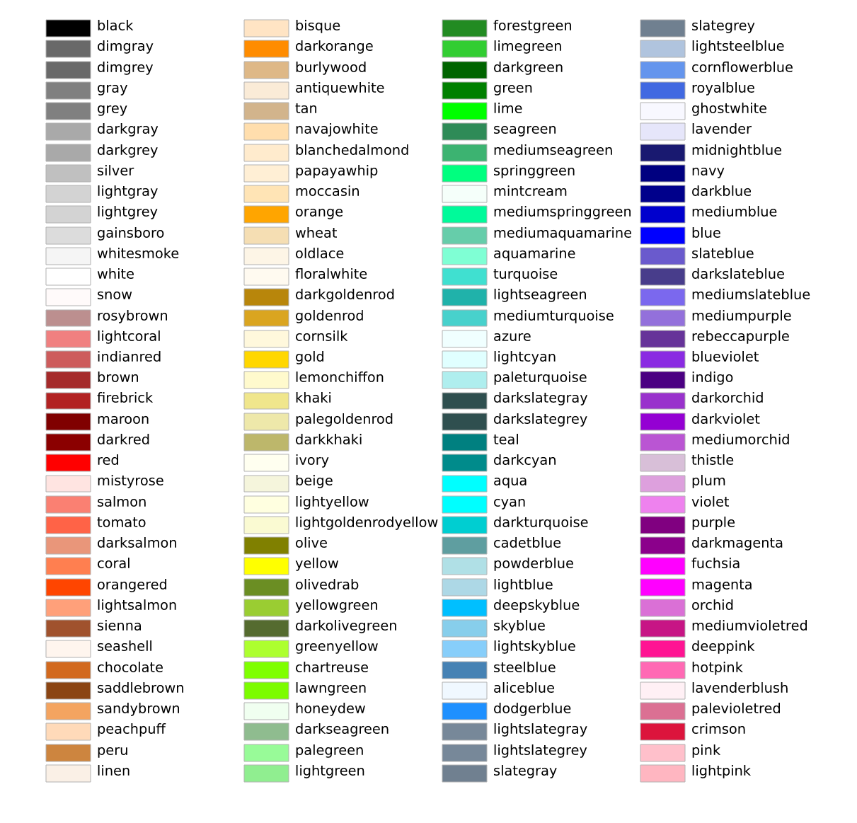
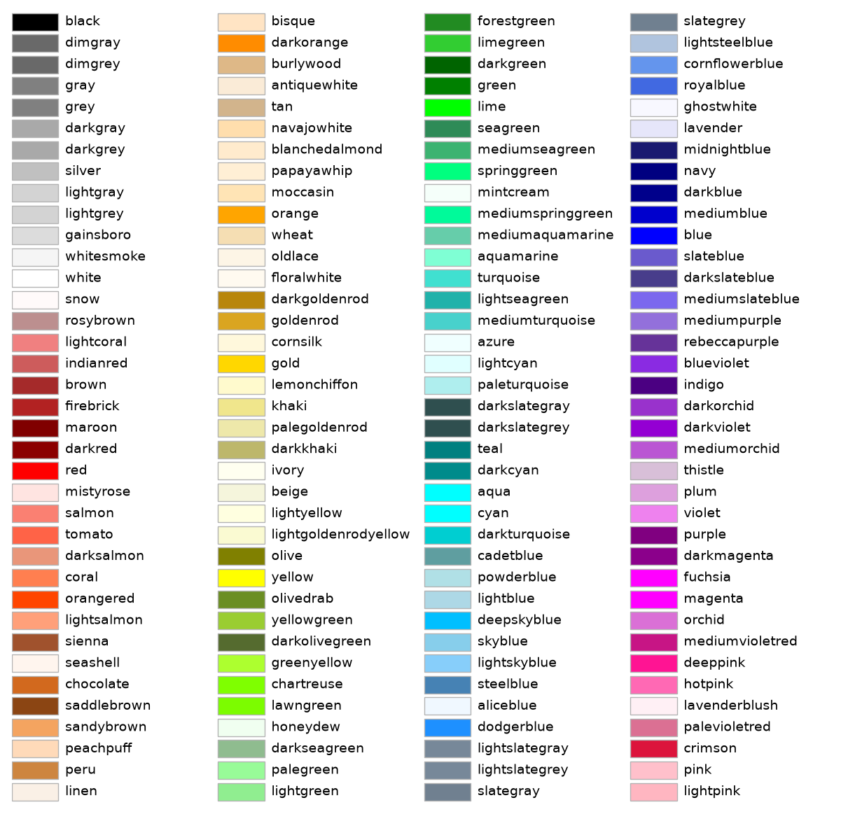
color/set_alpha
=================================
Source
"""
=================================
Ways to set a color's alpha value
=================================

Compare setting alpha by the *alpha* keyword argument and by one of the Matplotlib color
formats. Often, the *alpha* keyword is the only tool needed to add transparency to a
color. In some cases, the *(matplotlib_color, alpha)* color format provides an easy way
to fine-tune the appearance of a Figure.

"""

import matplotlib.pyplot as plt
import numpy as np

# Fixing random state for reproducibility.
np.random.seed(19680801)

fig, (ax1, ax2) = plt.subplots(ncols=2, figsize=(8, 4))

x_values = [n for n in range(20)]
y_values = np.random.randn(20)

facecolors = ['green' if y > 0 else 'red' for y in y_values]
edgecolors = facecolors

ax1.bar(x_values, y_values, color=facecolors, edgecolor=edgecolors, alpha=0.5)
ax1.set_title("Explicit 'alpha' keyword value\nshared by all bars and edges")


# Normalize y values to get distinct face alpha values.
abs_y = [abs(y) for y in y_values]
face_alphas = [n / max(abs_y) for n in abs_y]
edge_alphas = [1 - alpha for alpha in face_alphas]

colors_with_alphas = list(zip(facecolors, face_alphas))
edgecolors_with_alphas = list(zip(edgecolors, edge_alphas))

ax2.bar(x_values, y_values, color=colors_with_alphas,
        edgecolor=edgecolors_with_alphas)
ax2.set_title('Normalized alphas for\neach bar and each edge')

plt.show()

# %%
#
# .. admonition:: References
#
#    The use of the following functions, methods, classes and modules is shown
#    in this example:
#
#    - `matplotlib.axes.Axes.bar`
#    - `matplotlib.pyplot.subplots`
#
# .. tags::
#
#    styling: color
#    plot-type: bar
#    level: beginner
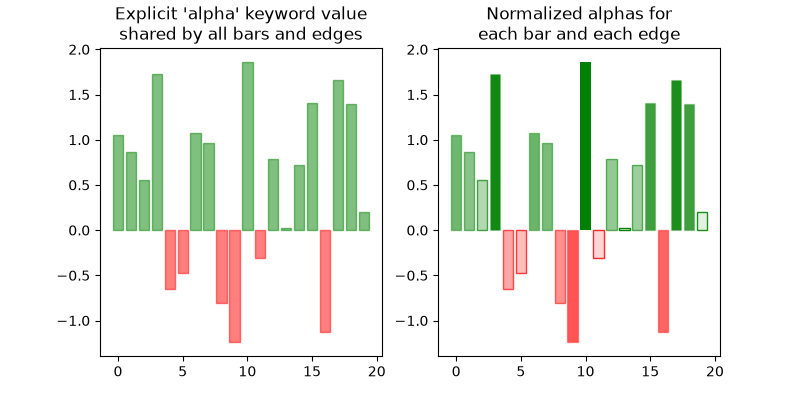
event_handling/close_event
===========
Source
"""
===========
Close event
===========

Example to show connecting events that occur when the figure closes.

.. note::
    This example exercises the interactive capabilities of Matplotlib, and this
    will not appear in the static documentation. Please run this code on your
    machine to see the interactivity.

    You can copy and paste individual parts, or download the entire example
    using the link at the bottom of the page.
"""
import matplotlib.pyplot as plt


def on_close(event):
    print('Closed Figure!')

fig = plt.figure()
fig.canvas.mpl_connect('close_event', on_close)

plt.text(0.35, 0.5, 'Close Me!', dict(size=30))
plt.show()
event_handling/coords_demo
===========================
Source
"""
===========================
Mouse move and click events
===========================

An example of how to interact with the plotting canvas by connecting to move
and click events.

.. note::
    This example exercises the interactive capabilities of Matplotlib, and this
    will not appear in the static documentation. Please run this code on your
    machine to see the interactivity.

    You can copy and paste individual parts, or download the entire example
    using the link at the bottom of the page.
"""

import matplotlib.pyplot as plt
import numpy as np

from matplotlib.backend_bases import MouseButton

t = np.arange(0.0, 1.0, 0.01)
s = np.sin(2 * np.pi * t)
fig, ax = plt.subplots()
ax.plot(t, s)


def on_move(event):
    if event.inaxes:
        print(f'data coords {event.xdata} {event.ydata},',
              f'pixel coords {event.x} {event.y}')


def on_click(event):
    if event.button is MouseButton.LEFT:
        print('disconnecting callback')
        plt.disconnect(binding_id)


binding_id = plt.connect('motion_notify_event', on_move)
plt.connect('button_press_event', on_click)

plt.show()
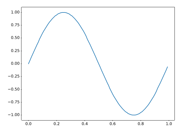
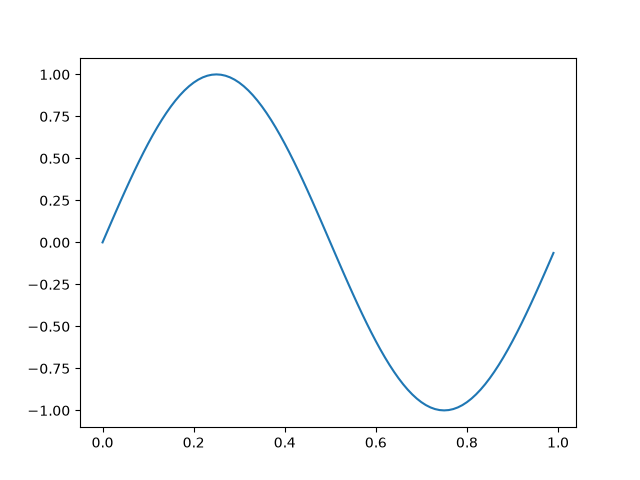
event_handling/cursor_demo
=================
Source
"""
=================
Cross-hair cursor
=================

This example adds a cross-hair as a data cursor.  The cross-hair is
implemented as regular line objects that are updated on mouse move.

We show three implementations:

1) A simple cursor implementation that redraws the figure on every mouse move.
   This is a bit slow, and you may notice some lag of the cross-hair movement.
2) A cursor that uses blitting for speedup of the rendering.
3) A cursor that snaps to data points.

Faster cursoring is possible using native GUI drawing, as in
:doc:`/gallery/user_interfaces/wxcursor_demo_sgskip`.

The mpldatacursor__ and mplcursors__ third-party packages can be used to
achieve a similar effect.

__ https://github.com/joferkington/mpldatacursor
__ https://github.com/anntzer/mplcursors

.. redirect-from:: /gallery/misc/cursor_demo
"""

import matplotlib.pyplot as plt
import numpy as np

from matplotlib.backend_bases import MouseEvent


class Cursor:
    """
    A cross hair cursor.
    """
    def __init__(self, ax):
        self.ax = ax
        self.horizontal_line = ax.axhline(color='k', lw=0.8, ls='--')
        self.vertical_line = ax.axvline(color='k', lw=0.8, ls='--')
        # text location in axes coordinates
        self.text = ax.text(0.72, 0.9, '', transform=ax.transAxes)

    def set_cross_hair_visible(self, visible):
        need_redraw = self.horizontal_line.get_visible() != visible
        self.horizontal_line.set_visible(visible)
        self.vertical_line.set_visible(visible)
        self.text.set_visible(visible)
        return need_redraw

    def on_mouse_move(self, event):
        if not event.inaxes:
            need_redraw = self.set_cross_hair_visible(False)
            if need_redraw:
                self.ax.figure.canvas.draw()
        else:
            self.set_cross_hair_visible(True)
            x, y = event.xdata, event.ydata
            # update the line positions
            self.horizontal_line.set_ydata([y])
            self.vertical_line.set_xdata([x])
            self.text.set_text(f'x={x:1.2f}, y={y:1.2f}')
            self.ax.figure.canvas.draw()


x = np.arange(0, 1, 0.01)
y = np.sin(2 * 2 * np.pi * x)

fig, ax = plt.subplots()
ax.set_title('Simple cursor')
ax.plot(x, y, 'o')
cursor = Cursor(ax)
fig.canvas.mpl_connect('motion_notify_event', cursor.on_mouse_move)

# Simulate a mouse move to (0.5, 0.5), needed for online docs
t = ax.transData
MouseEvent(
    "motion_notify_event", ax.figure.canvas, *t.transform((0.5, 0.5))
)._process()

# %%
# Faster redrawing using blitting
# """""""""""""""""""""""""""""""
# This technique stores the rendered plot as a background image. Only the
# changed artists (cross-hair lines and text) are rendered anew. They are
# combined with the background using blitting.
#
# This technique is significantly faster. It requires a bit more setup because
# the background has to be stored without the cross-hair lines (see
# ``create_new_background()``). Additionally, a new background has to be
# created whenever the figure changes. This is achieved by connecting to the
# ``'draw_event'``.


class BlittedCursor:
    """
    A cross-hair cursor using blitting for faster redraw.
    """
    def __init__(self, ax):
        self.ax = ax
        self.background = None
        self.horizontal_line = ax.axhline(color='k', lw=0.8, ls='--')
        self.vertical_line = ax.axvline(color='k', lw=0.8, ls='--')
        # text location in axes coordinates
        self.text = ax.text(0.72, 0.9, '', transform=ax.transAxes)
        self._creating_background = False
        ax.figure.canvas.mpl_connect('draw_event', self.on_draw)

    def on_draw(self, event):
        self.create_new_background()

    def set_cross_hair_visible(self, visible):
        need_redraw = self.horizontal_line.get_visible() != visible
        self.horizontal_line.set_visible(visible)
        self.vertical_line.set_visible(visible)
        self.text.set_visible(visible)
        return need_redraw

    def create_new_background(self):
        if self._creating_background:
            # discard calls triggered from within this function
            return
        self._creating_background = True
        self.set_cross_hair_visible(False)
        self.ax.figure.canvas.draw()
        self.background = self.ax.figure.canvas.copy_from_bbox(self.ax.bbox)
        self.set_cross_hair_visible(True)
        self._creating_background = False

    def on_mouse_move(self, event):
        if self.background is None:
            self.create_new_background()
        if not event.inaxes:
            need_redraw = self.set_cross_hair_visible(False)
            if need_redraw:
                self.ax.figure.canvas.restore_region(self.background)
                self.ax.figure.canvas.blit(self.ax.bbox)
        else:
            self.set_cross_hair_visible(True)
            # update the line positions
            x, y = event.xdata, event.ydata
            self.horizontal_line.set_ydata([y])
            self.vertical_line.set_xdata([x])
            self.text.set_text(f'x={x:1.2f}, y={y:1.2f}')

            self.ax.figure.canvas.restore_region(self.background)
            self.ax.draw_artist(self.horizontal_line)
            self.ax.draw_artist(self.vertical_line)
            self.ax.draw_artist(self.text)
            self.ax.figure.canvas.blit(self.ax.bbox)


x = np.arange(0, 1, 0.01)
y = np.sin(2 * 2 * np.pi * x)

fig, ax = plt.subplots()
ax.set_title('Blitted cursor')
ax.plot(x, y, 'o')
blitted_cursor = BlittedCursor(ax)
fig.canvas.mpl_connect('motion_notify_event', blitted_cursor.on_mouse_move)

# Simulate a mouse move to (0.5, 0.5), needed for online docs
t = ax.transData
MouseEvent(
    "motion_notify_event", ax.figure.canvas, *t.transform((0.5, 0.5))
)._process()

# %%
# Snapping to data points
# """""""""""""""""""""""
# The following cursor snaps its position to the data points of a `.Line2D`
# object.
#
# To save unnecessary redraws, the index of the last indicated data point is
# saved in ``self._last_index``. A redraw is only triggered when the mouse
# moves far enough so that another data point must be selected. This reduces
# the lag due to many redraws. Of course, blitting could still be added on top
# for additional speedup.


class SnappingCursor:
    """
    A cross-hair cursor that snaps to the data point of a line, which is
    closest to the *x* position of the cursor.

    For simplicity, this assumes that *x* values of the data are sorted.
    """
    def __init__(self, ax, line):
        self.ax = ax
        self.horizontal_line = ax.axhline(color='k', lw=0.8, ls='--')
        self.vertical_line = ax.axvline(color='k', lw=0.8, ls='--')
        self.x, self.y = line.get_data()
        self._last_index = None
        # text location in axes coords
        self.text = ax.text(0.72, 0.9, '', transform=ax.transAxes)

    def set_cross_hair_visible(self, visible):
        need_redraw = self.horizontal_line.get_visible() != visible
        self.horizontal_line.set_visible(visible)
        self.vertical_line.set_visible(visible)
        self.text.set_visible(visible)
        return need_redraw

    def on_mouse_move(self, event):
        if not event.inaxes:
            self._last_index = None
            need_redraw = self.set_cross_hair_visible(False)
            if need_redraw:
                self.ax.figure.canvas.draw()
        else:
            self.set_cross_hair_visible(True)
            x, y = event.xdata, event.ydata
            index = min(np.searchsorted(self.x, x), len(self.x) - 1)
            if index == self._last_index:
                return  # still on the same data point. Nothing to do.
            self._last_index = index
            x = self.x[index]
            y = self.y[index]
            # update the line positions
            self.horizontal_line.set_ydata([y])
            self.vertical_line.set_xdata([x])
            self.text.set_text(f'x={x:1.2f}, y={y:1.2f}')
            self.ax.figure.canvas.draw()


x = np.arange(0, 1, 0.01)
y = np.sin(2 * 2 * np.pi * x)

fig, ax = plt.subplots()
ax.set_title('Snapping cursor')
line, = ax.plot(x, y, 'o')
snap_cursor = SnappingCursor(ax, line)
fig.canvas.mpl_connect('motion_notify_event', snap_cursor.on_mouse_move)

# Simulate a mouse move to (0.5, 0.5), needed for online docs
t = ax.transData
MouseEvent(
    "motion_notify_event", ax.figure.canvas, *t.transform((0.5, 0.5))
)._process()

plt.show()
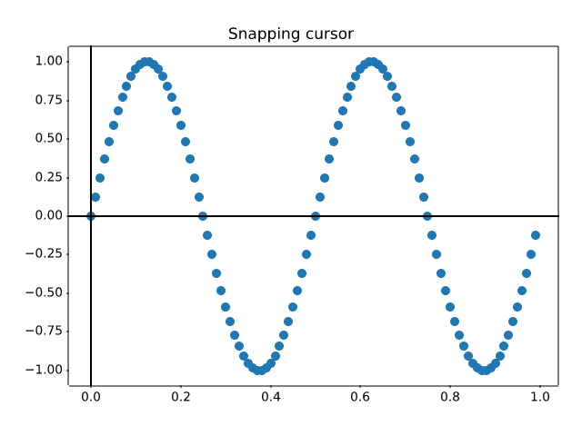
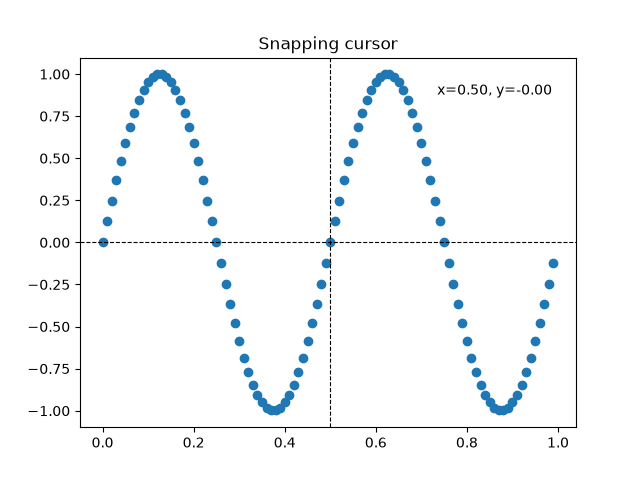
event_handling/data_browser
============
Source
"""
============
Data browser
============

Connecting data between multiple canvases.

This example covers how to interact data with multiple canvases. This
lets you select and highlight a point on one axis, and generating the
data of that point on the other axis.

.. note::
    This example exercises the interactive capabilities of Matplotlib, and this
    will not appear in the static documentation. Please run this code on your
    machine to see the interactivity.

    You can copy and paste individual parts, or download the entire example
    using the link at the bottom of the page.
"""
import numpy as np


class PointBrowser:
    """
    Click on a point to select and highlight it -- the data that
    generated the point will be shown in the lower Axes.  Use the 'n'
    and 'p' keys to browse through the next and previous points
    """

    def __init__(self):
        self.lastind = 0

        self.text = ax.text(0.05, 0.95, 'selected: none',
                            transform=ax.transAxes, va='top')
        self.selected, = ax.plot([xs[0]], [ys[0]], 'o', ms=12, alpha=0.4,
                                 color='yellow', visible=False)

    def on_press(self, event):
        if self.lastind is None:
            return
        if event.key not in ('n', 'p'):
            return
        if event.key == 'n':
            inc = 1
        else:
            inc = -1

        self.lastind += inc
        self.lastind = np.clip(self.lastind, 0, len(xs) - 1)
        self.update()

    def on_pick(self, event):

        if event.artist != line:
            return True

        N = len(event.ind)
        if not N:
            return True

        # the click locations
        x = event.mouseevent.xdata
        y = event.mouseevent.ydata

        distances = np.hypot(x - xs[event.ind], y - ys[event.ind])
        indmin = distances.argmin()
        dataind = event.ind[indmin]

        self.lastind = dataind
        self.update()

    def update(self):
        if self.lastind is None:
            return

        dataind = self.lastind

        ax2.clear()
        ax2.plot(X[dataind])

        ax2.text(0.05, 0.9, f'mu={xs[dataind]:1.3f}\nsigma={ys[dataind]:1.3f}',
                 transform=ax2.transAxes, va='top')
        ax2.set_ylim(-0.5, 1.5)
        self.selected.set_visible(True)
        self.selected.set_data([xs[dataind]], [ys[dataind]])

        self.text.set_text('selected: %d' % dataind)
        fig.canvas.draw()


if __name__ == '__main__':
    import matplotlib.pyplot as plt

    # Fixing random state for reproducibility
    np.random.seed(19680801)

    X = np.random.rand(100, 200)
    xs = np.mean(X, axis=1)
    ys = np.std(X, axis=1)

    fig, (ax, ax2) = plt.subplots(2, 1)
    ax.set_title('click on point to plot time series')
    line, = ax.plot(xs, ys, 'o', picker=True, pickradius=5)

    browser = PointBrowser()

    fig.canvas.mpl_connect('pick_event', browser.on_pick)
    fig.canvas.mpl_connect('key_press_event', browser.on_press)

    plt.show()
event_handling/figure_axes_enter_leave
==================================
Source
"""
==================================
Figure/Axes enter and leave events
==================================

Illustrate the figure and Axes enter and leave events by changing the
frame colors on enter and leave.

.. note::
    This example exercises the interactive capabilities of Matplotlib, and this
    will not appear in the static documentation. Please run this code on your
    machine to see the interactivity.

    You can copy and paste individual parts, or download the entire example
    using the link at the bottom of the page.
"""
import matplotlib.pyplot as plt


def on_enter_axes(event):
    print('enter_axes', event.inaxes)
    event.inaxes.patch.set_facecolor('yellow')
    event.canvas.draw()


def on_leave_axes(event):
    print('leave_axes', event.inaxes)
    event.inaxes.patch.set_facecolor('white')
    event.canvas.draw()


def on_enter_figure(event):
    print('enter_figure', event.canvas.figure)
    event.canvas.figure.patch.set_facecolor('red')
    event.canvas.draw()


def on_leave_figure(event):
    print('leave_figure', event.canvas.figure)
    event.canvas.figure.patch.set_facecolor('grey')
    event.canvas.draw()


fig, axs = plt.subplots(2, 1)
fig.suptitle('mouse hover over figure or Axes to trigger events')

fig.canvas.mpl_connect('figure_enter_event', on_enter_figure)
fig.canvas.mpl_connect('figure_leave_event', on_leave_figure)
fig.canvas.mpl_connect('axes_enter_event', on_enter_axes)
fig.canvas.mpl_connect('axes_leave_event', on_leave_axes)

plt.show()
event_handling/ginput_manual_clabel_sgskip
=====================
Source
"""
=====================
Interactive functions
=====================

This provides examples of uses of interactive functions, such as ginput,
waitforbuttonpress and manual clabel placement.

.. note::
    This example exercises the interactive capabilities of Matplotlib, and this
    will not appear in the static documentation. Please run this code on your
    machine to see the interactivity.

    You can copy and paste individual parts, or download the entire example
    using the link at the bottom of the page.
"""

import time

import matplotlib.pyplot as plt
import numpy as np


def tellme(s):
    print(s)
    plt.title(s, fontsize=16)
    plt.draw()

# %%
# Define a triangle by clicking three points


plt.figure()
plt.xlim(0, 1)
plt.ylim(0, 1)

tellme('You will define a triangle, click to begin')

plt.waitforbuttonpress()

while True:
    pts = []
    while len(pts) < 3:
        tellme('Select 3 corners with mouse')
        pts = np.asarray(plt.ginput(3, timeout=-1))
        if len(pts) < 3:
            tellme('Too few points, starting over')
            time.sleep(1)  # Wait a second

    ph = plt.fill(pts[:, 0], pts[:, 1], 'r', lw=2)

    tellme('Happy? Key click for yes, mouse click for no')

    if plt.waitforbuttonpress():
        break

    # Get rid of fill
    for p in ph:
        p.remove()


# %%
# Now contour according to distance from triangle
# corners - just an example

# Define a nice function of distance from individual pts
def f(x, y, pts):
    z = np.zeros_like(x)
    for p in pts:
        z = z + 1/(np.sqrt((x - p[0])**2 + (y - p[1])**2))
    return 1/z


X, Y = np.meshgrid(np.linspace(-1, 1, 51), np.linspace(-1, 1, 51))
Z = f(X, Y, pts)

CS = plt.contour(X, Y, Z, 20)

tellme('Use mouse to select contour label locations, middle button to finish')
CL = plt.clabel(CS, manual=True)

# %%
# Now do a zoom

tellme('Now do a nested zoom, click to begin')
plt.waitforbuttonpress()

while True:
    tellme('Select two corners of zoom, middle mouse button to finish')
    pts = plt.ginput(2, timeout=-1)
    if len(pts) < 2:
        break
    (x0, y0), (x1, y1) = pts
    xmin, xmax = sorted([x0, x1])
    ymin, ymax = sorted([y0, y1])
    plt.xlim(xmin, xmax)
    plt.ylim(ymin, ymax)

tellme('All Done!')
plt.show()
interactive or unparseable
event_handling/image_slices_viewer
============
Source
"""
============
Scroll event
============

In this example a scroll wheel event is used to scroll through 2D slices of
3D data.

.. note::
    This example exercises the interactive capabilities of Matplotlib, and this
    will not appear in the static documentation. Please run this code on your
    machine to see the interactivity.

    You can copy and paste individual parts, or download the entire example
    using the link at the bottom of the page.
"""

import matplotlib.pyplot as plt
import numpy as np


class IndexTracker:
    def __init__(self, ax, X):
        self.index = 0
        self.X = X
        self.ax = ax
        self.im = ax.imshow(self.X[:, :, self.index])
        self.update()

    def on_scroll(self, event):
        print(event.button, event.step)
        increment = 1 if event.button == 'up' else -1
        max_index = self.X.shape[-1] - 1
        self.index = np.clip(self.index + increment, 0, max_index)
        self.update()

    def update(self):
        self.im.set_data(self.X[:, :, self.index])
        self.ax.set_title(
            f'Use scroll wheel to navigate\nindex {self.index}')
        self.im.axes.figure.canvas.draw()


x, y, z = np.ogrid[-10:10:100j, -10:10:100j, 1:10:20j]
X = np.sin(x * y * z) / (x * y * z)

fig, ax = plt.subplots()
# create an IndexTracker and make sure it lives during the whole
# lifetime of the figure by assigning it to a variable
tracker = IndexTracker(ax, X)

fig.canvas.mpl_connect('scroll_event', tracker.on_scroll)
plt.show()
event_handling/keypress_demo
==============
Source
"""
==============
Keypress event
==============

Show how to connect to keypress events.

.. note::
    This example exercises the interactive capabilities of Matplotlib, and this
    will not appear in the static documentation. Please run this code on your
    machine to see the interactivity.

    You can copy and paste individual parts, or download the entire example
    using the link at the bottom of the page.
"""
import sys

import matplotlib.pyplot as plt
import numpy as np


def on_press(event):
    print('press', event.key)
    sys.stdout.flush()
    if event.key == 'x':
        visible = xl.get_visible()
        xl.set_visible(not visible)
        fig.canvas.draw()


# Fixing random state for reproducibility
np.random.seed(19680801)

fig, ax = plt.subplots()

fig.canvas.mpl_connect('key_press_event', on_press)

ax.plot(np.random.rand(12), np.random.rand(12), 'go')
xl = ax.set_xlabel('easy come, easy go')
ax.set_title('Press a key')
plt.show()
event_handling/lasso_demo
==========
Source
"""
==========
Lasso Demo
==========

Use a lasso to select a set of points and get the indices of the selected points.
A callback is used to change the color of the selected points.

.. note::
    This example exercises the interactive capabilities of Matplotlib, and this
    will not appear in the static documentation. Please run this code on your
    machine to see the interactivity.

    You can copy and paste individual parts, or download the entire example
    using the link at the bottom of the page.
"""

import matplotlib.pyplot as plt
import numpy as np

from matplotlib import colors as mcolors
from matplotlib import path
from matplotlib.collections import RegularPolyCollection
from matplotlib.widgets import Lasso


class LassoManager:
    def __init__(self, ax, data):
        # The information of whether a point has been selected or not is stored in the
        # collection's array (0 = out, 1 = in), which then gets colormapped to blue
        # (out) and red (in).
        self.collection = RegularPolyCollection(
            6, sizes=(100,), offset_transform=ax.transData,
            offsets=data, array=np.zeros(len(data)),
            clim=(0, 1), cmap=mcolors.ListedColormap(["tab:blue", "tab:red"]))
        ax.add_collection(self.collection)
        canvas = ax.figure.canvas
        canvas.mpl_connect('button_press_event', self.on_press)
        canvas.mpl_connect('button_release_event', self.on_release)

    def callback(self, verts):
        data = self.collection.get_offsets()
        self.collection.set_array(path.Path(verts).contains_points(data))
        canvas = self.collection.figure.canvas
        canvas.draw_idle()
        del self.lasso

    def on_press(self, event):
        canvas = self.collection.figure.canvas
        if event.inaxes is not self.collection.axes or canvas.widgetlock.locked():
            return
        self.lasso = Lasso(event.inaxes, (event.xdata, event.ydata), self.callback)
        canvas.widgetlock(self.lasso)  # acquire a lock on the widget drawing

    def on_release(self, event):
        canvas = self.collection.figure.canvas
        if hasattr(self, 'lasso') and canvas.widgetlock.isowner(self.lasso):
            canvas.widgetlock.release(self.lasso)


if __name__ == '__main__':
    np.random.seed(19680801)
    ax = plt.figure().add_subplot(
        xlim=(0, 1), ylim=(0, 1), title='Lasso points using left mouse button')
    manager = LassoManager(ax, np.random.rand(100, 2))
    plt.show()
event_handling/legend_picking
==============
Source
"""
==============
Legend picking
==============

Enable picking on the legend to toggle the original line on and off

.. note::
    This example exercises the interactive capabilities of Matplotlib, and this
    will not appear in the static documentation. Please run this code on your
    machine to see the interactivity.

    You can copy and paste individual parts, or download the entire example
    using the link at the bottom of the page.
"""

import matplotlib.pyplot as plt
import numpy as np

t = np.linspace(0, 1)
y1 = 2 * np.sin(2 * np.pi * t)
y2 = 4 * np.sin(2 * np.pi * 2 * t)

fig, ax = plt.subplots()
ax.set_title('Click on legend line to toggle line on/off')
(line1, ) = ax.plot(t, y1, lw=2, label='1 Hz')
(line2, ) = ax.plot(t, y2, lw=2, label='2 Hz')
leg = ax.legend(fancybox=True, shadow=True)

lines = [line1, line2]
map_legend_to_ax = {}  # Will map legend lines to original lines.

pickradius = 5  # Points (Pt). How close the click needs to be to trigger an event.

for legend_line, ax_line in zip(leg.get_lines(), lines):
    legend_line.set_picker(pickradius)  # Enable picking on the legend line.
    map_legend_to_ax[legend_line] = ax_line


def on_pick(event):
    # On the pick event, find the original line corresponding to the legend
    # proxy line, and toggle its visibility.
    legend_line = event.artist

    # Do nothing if the source of the event is not a legend line.
    if legend_line not in map_legend_to_ax:
        return

    ax_line = map_legend_to_ax[legend_line]
    visible = not ax_line.get_visible()
    ax_line.set_visible(visible)
    # Change the alpha on the line in the legend, so we can see what lines
    # have been toggled.
    legend_line.set_alpha(1.0 if visible else 0.2)
    fig.canvas.draw()


fig.canvas.mpl_connect('pick_event', on_pick)

# Works even if the legend is draggable. This is independent from picking legend lines.
leg.set_draggable(True)

plt.show()
event_handling/looking_glass
=============
Source
"""
=============
Looking glass
=============

Example using mouse events to simulate a looking glass for inspecting data.

.. note::
    This example exercises the interactive capabilities of Matplotlib, and this
    will not appear in the static documentation. Please run this code on your
    machine to see the interactivity.

    You can copy and paste individual parts, or download the entire example
    using the link at the bottom of the page.
"""
import matplotlib.pyplot as plt
import numpy as np

import matplotlib.patches as patches

# Fixing random state for reproducibility
np.random.seed(19680801)

x, y = np.random.rand(2, 200)

fig, ax = plt.subplots()
circ = patches.Circle((0.5, 0.5), 0.25, alpha=0.8, fc='yellow')
ax.add_patch(circ)


ax.plot(x, y, alpha=0.2)
line, = ax.plot(x, y, alpha=1.0, clip_path=circ)
ax.set_title("Left click and drag to move looking glass")


class EventHandler:
    def __init__(self):
        fig.canvas.mpl_connect('button_press_event', self.on_press)
        fig.canvas.mpl_connect('button_release_event', self.on_release)
        fig.canvas.mpl_connect('motion_notify_event', self.on_move)
        self.x0, self.y0 = circ.center
        self.pressevent = None

    def on_press(self, event):
        if event.inaxes != ax:
            return

        if not circ.contains(event)[0]:
            return

        self.pressevent = event

    def on_release(self, event):
        self.pressevent = None
        self.x0, self.y0 = circ.center

    def on_move(self, event):
        if self.pressevent is None or event.inaxes != self.pressevent.inaxes:
            return

        dx = event.xdata - self.pressevent.xdata
        dy = event.ydata - self.pressevent.ydata
        circ.center = self.x0 + dx, self.y0 + dy
        line.set_clip_path(circ)
        fig.canvas.draw()

handler = EventHandler()
plt.show()
event_handling/path_editor
===========
Source
"""
===========
Path editor
===========

Sharing events across GUIs.

This example demonstrates a cross-GUI application using Matplotlib event
handling to interact with and modify objects on the canvas.

.. note::
    This example exercises the interactive capabilities of Matplotlib, and this
    will not appear in the static documentation. Please run this code on your
    machine to see the interactivity.

    You can copy and paste individual parts, or download the entire example
    using the link at the bottom of the page.
"""

import matplotlib.pyplot as plt
import numpy as np

from matplotlib.backend_bases import MouseButton
from matplotlib.patches import PathPatch
from matplotlib.path import Path

fig, ax = plt.subplots()

pathdata = [
    (Path.MOVETO, (1.58, -2.57)),
    (Path.CURVE4, (0.35, -1.1)),
    (Path.CURVE4, (-1.75, 2.0)),
    (Path.CURVE4, (0.375, 2.0)),
    (Path.LINETO, (0.85, 1.15)),
    (Path.CURVE4, (2.2, 3.2)),
    (Path.CURVE4, (3, 0.05)),
    (Path.CURVE4, (2.0, -0.5)),
    (Path.CLOSEPOLY, (1.58, -2.57)),
]

codes, verts = zip(*pathdata)
path = Path(verts, codes)
patch = PathPatch(
    path, facecolor='green', edgecolor='yellow', alpha=0.5)
ax.add_patch(patch)


class PathInteractor:
    """
    A path editor.

    Press 't' to toggle vertex markers on and off.  When vertex markers are on,
    they can be dragged with the mouse.
    """

    showverts = True
    epsilon = 5  # max pixel distance to count as a vertex hit

    def __init__(self, pathpatch):

        self.ax = pathpatch.axes
        canvas = self.ax.figure.canvas
        self.pathpatch = pathpatch
        self.pathpatch.set_animated(True)

        x, y = zip(*self.pathpatch.get_path().vertices)

        self.line, = ax.plot(
            x, y, marker='o', markerfacecolor='r', animated=True)

        self._ind = None  # the active vertex

        canvas.mpl_connect('draw_event', self.on_draw)
        canvas.mpl_connect('button_press_event', self.on_button_press)
        canvas.mpl_connect('key_press_event', self.on_key_press)
        canvas.mpl_connect('button_release_event', self.on_button_release)
        canvas.mpl_connect('motion_notify_event', self.on_mouse_move)
        self.canvas = canvas

    def get_ind_under_point(self, event):
        """
        Return the index of the point closest to the event position or *None*
        if no point is within ``self.epsilon`` to the event position.
        """
        xy = self.pathpatch.get_path().vertices
        xyt = self.pathpatch.get_transform().transform(xy)  # to display coords
        xt, yt = xyt[:, 0], xyt[:, 1]
        d = np.sqrt((xt - event.x)**2 + (yt - event.y)**2)
        ind = d.argmin()
        return ind if d[ind] < self.epsilon else None

    def on_draw(self, event):
        """Callback for draws."""
        self.background = self.canvas.copy_from_bbox(self.ax.bbox)
        self.ax.draw_artist(self.pathpatch)
        self.ax.draw_artist(self.line)

    def on_button_press(self, event):
        """Callback for mouse button presses."""
        if (event.inaxes is None
                or event.button != MouseButton.LEFT
                or not self.showverts):
            return
        self._ind = self.get_ind_under_point(event)

    def on_button_release(self, event):
        """Callback for mouse button releases."""
        if (event.button != MouseButton.LEFT
                or not self.showverts):
            return
        self._ind = None

    def on_key_press(self, event):
        """Callback for key presses."""
        if not event.inaxes:
            return
        if event.key == 't':
            self.showverts = not self.showverts
            self.line.set_visible(self.showverts)
            if not self.showverts:
                self._ind = None
        self.canvas.draw()

    def on_mouse_move(self, event):
        """Callback for mouse movements."""
        if (self._ind is None
                or event.inaxes is None
                or event.button != MouseButton.LEFT
                or not self.showverts):
            return

        vertices = self.pathpatch.get_path().vertices

        vertices[self._ind] = event.xdata, event.ydata
        self.line.set_data(zip(*vertices))

        self.canvas.restore_region(self.background)
        self.ax.draw_artist(self.pathpatch)
        self.ax.draw_artist(self.line)
        self.canvas.blit(self.ax.bbox)


interactor = PathInteractor(patch)
ax.set_title('drag vertices to update path')
ax.set_xlim(-3, 4)
ax.set_ylim(-3, 4)

plt.show()
event_handling/pick_event_demo
===============
Source
"""
===============
Pick event demo
===============

You can enable picking by setting the "picker" property of an artist
(for example, a Matplotlib Line2D, Text, Patch, Polygon, AxesImage,
etc.)

There are a variety of meanings of the picker property:

* *None* - picking is disabled for this artist (default)

* bool - if *True* then picking will be enabled and the artist will fire a pick
  event if the mouse event is over the artist.

  Setting ``pickradius`` will add an epsilon tolerance in points and the artist
  will fire off an event if its data is within epsilon of the mouse event.  For
  some artists like lines and patch collections, the artist may provide
  additional data to the pick event that is generated, for example, the indices
  of the data within epsilon of the pick event

* function - if picker is callable, it is a user supplied function which
  determines whether the artist is hit by the mouse event. ::

     hit, props = picker(artist, mouseevent)

  to determine the hit test.  If the mouse event is over the artist, return
  hit=True and props is a dictionary of properties you want added to the
  PickEvent attributes.

After you have enabled an artist for picking by setting the "picker"
property, you need to connect to the figure canvas pick_event to get
pick callbacks on mouse press events.  For example, ::

  def pick_handler(event):
      mouseevent = event.mouseevent
      artist = event.artist
      # now do something with this...


The pick event (matplotlib.backend_bases.PickEvent) which is passed to
your callback is always fired with two attributes:

mouseevent
  the mouse event that generate the pick event.

  The mouse event in turn has attributes like x and y (the coordinates in
  display space, such as pixels from left, bottom) and xdata, ydata (the
  coords in data space).  Additionally, you can get information about
  which buttons were pressed, which keys were pressed, which Axes
  the mouse is over, etc.  See matplotlib.backend_bases.MouseEvent
  for details.

artist
  the matplotlib.artist that generated the pick event.

Additionally, certain artists like Line2D and PatchCollection may
attach additional metadata like the indices into the data that meet
the picker criteria (for example, all the points in the line that are within
the specified epsilon tolerance)

The examples below illustrate each of these methods.

.. note::
    These examples exercises the interactive capabilities of Matplotlib, and
    this will not appear in the static documentation. Please run this code on
    your machine to see the interactivity.

    You can copy and paste individual parts, or download the entire example
    using the link at the bottom of the page.
"""

import matplotlib.pyplot as plt
import numpy as np
from numpy.random import rand

from matplotlib.image import AxesImage
from matplotlib.lines import Line2D
from matplotlib.patches import Rectangle
from matplotlib.text import Text

# Fixing random state for reproducibility
np.random.seed(19680801)


# %%
# Simple picking, lines, rectangles and text
# ------------------------------------------

fig, (ax1, ax2) = plt.subplots(2, 1)
ax1.set_title('click on points, rectangles or text', picker=True)
ax1.set_ylabel('ylabel', picker=True, bbox=dict(facecolor='red'))
line, = ax1.plot(rand(100), 'o', picker=True, pickradius=5)

# Pick the rectangle.
ax2.bar(range(10), rand(10), picker=True)
for label in ax2.get_xticklabels():  # Make the xtick labels pickable.
    label.set_picker(True)


def onpick1(event):
    if isinstance(event.artist, Line2D):
        thisline = event.artist
        xdata = thisline.get_xdata()
        ydata = thisline.get_ydata()
        ind = event.ind
        print('onpick1 line:', np.column_stack([xdata[ind], ydata[ind]]))
    elif isinstance(event.artist, Rectangle):
        patch = event.artist
        print('onpick1 patch:', patch.get_path())
    elif isinstance(event.artist, Text):
        text = event.artist
        print('onpick1 text:', text.get_text())


fig.canvas.mpl_connect('pick_event', onpick1)


# %%
# Picking with a custom hit test function
# ---------------------------------------
# You can define custom pickers by setting picker to a callable function. The
# function has the signature::
#
#  hit, props = func(artist, mouseevent)
#
# to determine the hit test. If the mouse event is over the artist, return
# ``hit=True`` and ``props`` is a dictionary of properties you want added to
# the `.PickEvent` attributes.

def line_picker(line, mouseevent):
    """
    Find the points within a certain distance from the mouseclick in
    data coords and attach some extra attributes, pickx and picky
    which are the data points that were picked.
    """
    if mouseevent.xdata is None:
        return False, dict()
    xdata = line.get_xdata()
    ydata = line.get_ydata()
    maxd = 0.05
    d = np.sqrt(
        (xdata - mouseevent.xdata)**2 + (ydata - mouseevent.ydata)**2)

    ind, = np.nonzero(d <= maxd)
    if len(ind):
        pickx = xdata[ind]
        picky = ydata[ind]
        props = dict(ind=ind, pickx=pickx, picky=picky)
        return True, props
    else:
        return False, dict()


def onpick2(event):
    print('onpick2 line:', event.pickx, event.picky)


fig, ax = plt.subplots()
ax.set_title('custom picker for line data')
line, = ax.plot(rand(100), rand(100), 'o', picker=line_picker)
fig.canvas.mpl_connect('pick_event', onpick2)


# %%
# Picking on a scatter plot
# -------------------------
# A scatter plot is backed by a `~matplotlib.collections.PathCollection`.

x, y, c, s = rand(4, 100)


def onpick3(event):
    ind = event.ind
    print('onpick3 scatter:', ind, x[ind], y[ind])


fig, ax = plt.subplots()
ax.scatter(x, y, 100*s, c, picker=True)
fig.canvas.mpl_connect('pick_event', onpick3)


# %%
# Picking images
# --------------
# Images plotted using `.Axes.imshow` are `~matplotlib.image.AxesImage`
# objects.

fig, ax = plt.subplots()
ax.imshow(rand(10, 5), extent=(1, 2, 1, 2), picker=True)
ax.imshow(rand(5, 10), extent=(3, 4, 1, 2), picker=True)
ax.imshow(rand(20, 25), extent=(1, 2, 3, 4), picker=True)
ax.imshow(rand(30, 12), extent=(3, 4, 3, 4), picker=True)
ax.set(xlim=(0, 5), ylim=(0, 5))


def onpick4(event):
    artist = event.artist
    if isinstance(artist, AxesImage):
        im = artist
        A = im.get_array()
        print('onpick4 image', A.shape)


fig.canvas.mpl_connect('pick_event', onpick4)

plt.show()
event_handling/pick_event_demo2
=================
Source
"""
=================
Pick event demo 2
=================

Compute the mean (mu) and standard deviation (sigma) of 100 data sets and plot
mu vs. sigma.  When you click on one of the (mu, sigma) points, plot the raw
data from the dataset that generated this point.

.. note::
    This example exercises the interactive capabilities of Matplotlib, and this
    will not appear in the static documentation. Please run this code on your
    machine to see the interactivity.

    You can copy and paste individual parts, or download the entire example
    using the link at the bottom of the page.
"""
import matplotlib.pyplot as plt
import numpy as np

# Fixing random state for reproducibility
np.random.seed(19680801)

X = np.random.rand(100, 1000)
xs = np.mean(X, axis=1)
ys = np.std(X, axis=1)

fig, ax = plt.subplots()
ax.set_title('click on point to plot time series')
line, = ax.plot(xs, ys, 'o', picker=True, pickradius=5)


def onpick(event):

    if event.artist != line:
        return

    N = len(event.ind)
    if not N:
        return

    figi, axs = plt.subplots(N, squeeze=False)
    for ax, dataind in zip(axs.flat, event.ind):
        ax.plot(X[dataind])
        ax.text(.05, .9, f'mu={xs[dataind]:1.3f}\nsigma={ys[dataind]:1.3f}',
                transform=ax.transAxes, va='top')
        ax.set_ylim(-0.5, 1.5)
    figi.show()


fig.canvas.mpl_connect('pick_event', onpick)

plt.show()
event_handling/poly_editor
==============
Source
"""
==============
Polygon editor
==============

This is an example to show how to build cross-GUI applications using
Matplotlib event handling to interact with objects on the canvas.

.. note::
    This example exercises the interactive capabilities of Matplotlib, and this
    will not appear in the static documentation. Please run this code on your
    machine to see the interactivity.

    You can copy and paste individual parts, or download the entire example
    using the link at the bottom of the page.
"""

import numpy as np

from matplotlib.artist import Artist
from matplotlib.lines import Line2D


def dist_point_to_segment(p, s0, s1):
    """
    Get the distance from the point *p* to the segment (*s0*, *s1*), where
    *p*, *s0*, *s1* are ``[x, y]`` arrays.
    """
    s01 = s1 - s0
    s0p = p - s0
    if (s01 == 0).all():
        return np.hypot(*s0p)
    # Project onto segment, without going past segment ends.
    p1 = s0 + np.clip((s0p @ s01) / (s01 @ s01), 0, 1) * s01
    return np.hypot(*(p - p1))


class PolygonInteractor:
    """
    A polygon editor.

    Key-bindings

      't' toggle vertex markers on and off.  When vertex markers are on,
          you can move them, delete them

      'd' delete the vertex under point

      'i' insert a vertex at point.  You must be within epsilon of the
          line connecting two existing vertices

    """

    showverts = True
    epsilon = 5  # max pixel distance to count as a vertex hit

    def __init__(self, ax, poly):
        if poly.figure is None:
            raise RuntimeError('You must first add the polygon to a figure '
                               'or canvas before defining the interactor')
        self.ax = ax
        canvas = poly.figure.canvas
        self.poly = poly

        x, y = zip(*self.poly.xy)
        self.line = Line2D(x, y,
                           marker='o', markerfacecolor='r',
                           animated=True)
        self.ax.add_line(self.line)

        self.cid = self.poly.add_callback(self.poly_changed)
        self._ind = None  # the active vert

        canvas.mpl_connect('draw_event', self.on_draw)
        canvas.mpl_connect('button_press_event', self.on_button_press)
        canvas.mpl_connect('key_press_event', self.on_key_press)
        canvas.mpl_connect('button_release_event', self.on_button_release)
        canvas.mpl_connect('motion_notify_event', self.on_mouse_move)
        self.canvas = canvas

    def on_draw(self, event):
        self.background = self.canvas.copy_from_bbox(self.ax.bbox)
        self.ax.draw_artist(self.poly)
        self.ax.draw_artist(self.line)
        # do not need to blit here, this will fire before the screen is
        # updated

    def poly_changed(self, poly):
        """This method is called whenever the pathpatch object is called."""
        # only copy the artist props to the line (except visibility)
        vis = self.line.get_visible()
        Artist.update_from(self.line, poly)
        self.line.set_visible(vis)  # don't use the poly visibility state

    def get_ind_under_point(self, event):
        """
        Return the index of the point closest to the event position or *None*
        if no point is within ``self.epsilon`` to the event position.
        """
        # display coords
        xy = np.asarray(self.poly.xy)
        xyt = self.poly.get_transform().transform(xy)
        xt, yt = xyt[:, 0], xyt[:, 1]
        d = np.hypot(xt - event.x, yt - event.y)
        indseq, = np.nonzero(d == d.min())
        ind = indseq[0]

        if d[ind] >= self.epsilon:
            ind = None

        return ind

    def on_button_press(self, event):
        """Callback for mouse button presses."""
        if not self.showverts:
            return
        if event.inaxes is None:
            return
        if event.button != 1:
            return
        self._ind = self.get_ind_under_point(event)

    def on_button_release(self, event):
        """Callback for mouse button releases."""
        if not self.showverts:
            return
        if event.button != 1:
            return
        self._ind = None

    def on_key_press(self, event):
        """Callback for key presses."""
        if not event.inaxes:
            return
        if event.key == 't':
            self.showverts = not self.showverts
            self.line.set_visible(self.showverts)
            if not self.showverts:
                self._ind = None
        elif event.key == 'd':
            ind = self.get_ind_under_point(event)
            if ind is not None:
                self.poly.xy = np.delete(self.poly.xy,
                                         ind, axis=0)
                self.line.set_data(zip(*self.poly.xy))
        elif event.key == 'i':
            xys = self.poly.get_transform().transform(self.poly.xy)
            p = event.x, event.y  # display coords
            for i in range(len(xys) - 1):
                s0 = xys[i]
                s1 = xys[i + 1]
                d = dist_point_to_segment(p, s0, s1)
                if d <= self.epsilon:
                    self.poly.xy = np.insert(
                        self.poly.xy, i+1,
                        [event.xdata, event.ydata],
                        axis=0)
                    self.line.set_data(zip(*self.poly.xy))
                    break
        if self.line.stale:
            self.canvas.draw_idle()

    def on_mouse_move(self, event):
        """Callback for mouse movements."""
        if not self.showverts:
            return
        if self._ind is None:
            return
        if event.inaxes is None:
            return
        if event.button != 1:
            return
        x, y = event.xdata, event.ydata

        self.poly.xy[self._ind] = x, y
        if self._ind == 0:
            self.poly.xy[-1] = x, y
        elif self._ind == len(self.poly.xy) - 1:
            self.poly.xy[0] = x, y
        self.line.set_data(zip(*self.poly.xy))

        self.canvas.restore_region(self.background)
        self.ax.draw_artist(self.poly)
        self.ax.draw_artist(self.line)
        self.canvas.blit(self.ax.bbox)


if __name__ == '__main__':
    import matplotlib.pyplot as plt

    from matplotlib.patches import Polygon

    theta = np.arange(0, 2*np.pi, 0.1)
    r = 1.5

    xs = r * np.cos(theta)
    ys = r * np.sin(theta)

    poly = Polygon(np.column_stack([xs, ys]), animated=True)

    fig, ax = plt.subplots()
    ax.add_patch(poly)
    p = PolygonInteractor(ax, poly)

    ax.set_title('Click and drag a point to move it')
    ax.set_xlim(-2, 2)
    ax.set_ylim(-2, 2)
    plt.show()
event_handling/pong_sgskip
====
Source
"""
====
Pong
====

A Matplotlib based game of Pong illustrating one way to write interactive
animations that are easily ported to multiple backends.

.. note::
    This example exercises the interactive capabilities of Matplotlib, and this
    will not appear in the static documentation. Please run this code on your
    machine to see the interactivity.

    You can copy and paste individual parts, or download the entire example
    using the link at the bottom of the page.
"""

import time

import matplotlib.pyplot as plt
import numpy as np
from numpy.random import randint, randn

from matplotlib.font_manager import FontProperties

instructions = """
Player A:       Player B:
  'e'      up     'i'
  'd'     down    'k'

press 't' -- close these instructions
            (animation will be much faster)
press 'a' -- add a puck
press 'A' -- remove a puck
press '1' -- slow down all pucks
press '2' -- speed up all pucks
press '3' -- slow down distractors
press '4' -- speed up distractors
press ' ' -- reset the first puck
press 'n' -- toggle distractors on/off
press 'g' -- toggle the game on/off

  """


class Pad:
    def __init__(self, disp, x, y, type='l'):
        self.disp = disp
        self.x = x
        self.y = y
        self.w = .3
        self.score = 0
        self.xoffset = 0.3
        self.yoffset = 0.1
        if type == 'r':
            self.xoffset *= -1.0

        if type == 'l' or type == 'r':
            self.signx = -1.0
            self.signy = 1.0
        else:
            self.signx = 1.0
            self.signy = -1.0

    def contains(self, loc):
        return self.disp.get_bbox().contains(loc.x, loc.y)


class Puck:
    def __init__(self, disp, pad, field):
        self.vmax = .2
        self.disp = disp
        self.field = field
        self._reset(pad)

    def _reset(self, pad):
        self.x = pad.x + pad.xoffset
        if pad.y < 0:
            self.y = pad.y + pad.yoffset
        else:
            self.y = pad.y - pad.yoffset
        self.vx = pad.x - self.x
        self.vy = pad.y + pad.w/2 - self.y
        self._speedlimit()
        self._slower()
        self._slower()

    def update(self, pads):
        self.x += self.vx
        self.y += self.vy
        for pad in pads:
            if pad.contains(self):
                self.vx *= 1.2 * pad.signx
                self.vy *= 1.2 * pad.signy
        fudge = .001
        # probably cleaner with something like...
        if self.x < fudge:
            pads[1].score += 1
            self._reset(pads[0])
            return True
        if self.x > 7 - fudge:
            pads[0].score += 1
            self._reset(pads[1])
            return True
        if self.y < -1 + fudge or self.y > 1 - fudge:
            self.vy *= -1.0
            # add some randomness, just to make it interesting
            self.vy -= (randn()/300.0 + 1/300.0) * np.sign(self.vy)
        self._speedlimit()
        return False

    def _slower(self):
        self.vx /= 5.0
        self.vy /= 5.0

    def _faster(self):
        self.vx *= 5.0
        self.vy *= 5.0

    def _speedlimit(self):
        if self.vx > self.vmax:
            self.vx = self.vmax
        if self.vx < -self.vmax:
            self.vx = -self.vmax

        if self.vy > self.vmax:
            self.vy = self.vmax
        if self.vy < -self.vmax:
            self.vy = -self.vmax


class Game:
    def __init__(self, ax):
        # create the initial line
        self.ax = ax
        ax.xaxis.set_visible(False)
        ax.set_xlim(0, 7)
        ax.yaxis.set_visible(False)
        ax.set_ylim(-1, 1)
        pad_a_x = 0
        pad_b_x = .50
        pad_a_y = pad_b_y = .30
        pad_b_x += 6.3

        # pads
        pA, = self.ax.barh(pad_a_y, .2,
                           height=.3, color='k', alpha=.5, edgecolor='b',
                           lw=2, label="Player B",
                           animated=True)
        pB, = self.ax.barh(pad_b_y, .2,
                           height=.3, left=pad_b_x, color='k', alpha=.5,
                           edgecolor='r', lw=2, label="Player A",
                           animated=True)

        # distractors
        self.x = np.arange(0, 2.22*np.pi, 0.01)
        self.line, = self.ax.plot(self.x, np.sin(self.x), "r",
                                  animated=True, lw=4)
        self.line2, = self.ax.plot(self.x, np.cos(self.x), "g",
                                   animated=True, lw=4)
        self.line3, = self.ax.plot(self.x, np.cos(self.x), "g",
                                   animated=True, lw=4)
        self.line4, = self.ax.plot(self.x, np.cos(self.x), "r",
                                   animated=True, lw=4)

        # center line
        self.centerline, = self.ax.plot([3.5, 3.5], [1, -1], 'k',
                                        alpha=.5, animated=True, lw=8)

        # puck (s)
        self.puckdisp = self.ax.scatter([1], [1], label='_nolegend_',
                                        s=200, c='g',
                                        alpha=.9, animated=True)

        self.canvas = self.ax.figure.canvas
        self.background = None
        self.cnt = 0
        self.distract = True
        self.res = 100.0
        self.on = False
        self.inst = True    # show instructions from the beginning
        self.pads = [Pad(pA, pad_a_x, pad_a_y),
                     Pad(pB, pad_b_x, pad_b_y, 'r')]
        self.pucks = []
        self.i = self.ax.annotate(instructions, (.5, 0.5),
                                  name='monospace',
                                  verticalalignment='center',
                                  horizontalalignment='center',
                                  multialignment='left',
                                  xycoords='axes fraction',
                                  animated=False)
        self.canvas.mpl_connect('key_press_event', self.on_key_press)

    def draw(self):
        draw_artist = self.ax.draw_artist
        if self.background is None:
            self.background = self.canvas.copy_from_bbox(self.ax.bbox)

        # restore the clean slate background
        self.canvas.restore_region(self.background)

        # show the distractors
        if self.distract:
            self.line.set_ydata(np.sin(self.x + self.cnt/self.res))
            self.line2.set_ydata(np.cos(self.x - self.cnt/self.res))
            self.line3.set_ydata(np.tan(self.x + self.cnt/self.res))
            self.line4.set_ydata(np.tan(self.x - self.cnt/self.res))
            draw_artist(self.line)
            draw_artist(self.line2)
            draw_artist(self.line3)
            draw_artist(self.line4)

        # pucks and pads
        if self.on:
            self.ax.draw_artist(self.centerline)
            for pad in self.pads:
                pad.disp.set_y(pad.y)
                pad.disp.set_x(pad.x)
                self.ax.draw_artist(pad.disp)

            for puck in self.pucks:
                if puck.update(self.pads):
                    # we only get here if someone scored
                    self.pads[0].disp.set_label(f"   {self.pads[0].score}")
                    self.pads[1].disp.set_label(f"   {self.pads[1].score}")
                    self.ax.legend(loc='center', framealpha=.2,
                                   facecolor='0.5',
                                   prop=FontProperties(size='xx-large',
                                                       weight='bold'))

                    self.background = None
                    self.ax.figure.canvas.draw_idle()
                    return
                puck.disp.set_offsets([[puck.x, puck.y]])
                self.ax.draw_artist(puck.disp)

        # just redraw the Axes rectangle
        self.canvas.blit(self.ax.bbox)
        self.canvas.flush_events()
        if self.cnt == 50000:
            # just so we don't get carried away
            print("...and you've been playing for too long!!!")
            plt.close()

        self.cnt += 1

    def on_key_press(self, event):
        if event.key == '3':
            self.res *= 5.0
        if event.key == '4':
            self.res /= 5.0

        if event.key == 'e':
            self.pads[0].y += .1
            if self.pads[0].y > 1 - .3:
                self.pads[0].y = 1 - .3
        if event.key == 'd':
            self.pads[0].y -= .1
            if self.pads[0].y < -1:
                self.pads[0].y = -1

        if event.key == 'i':
            self.pads[1].y += .1
            if self.pads[1].y > 1 - .3:
                self.pads[1].y = 1 - .3
        if event.key == 'k':
            self.pads[1].y -= .1
            if self.pads[1].y < -1:
                self.pads[1].y = -1

        if event.key == 'a':
            self.pucks.append(Puck(self.puckdisp,
                                   self.pads[randint(2)],
                                   self.ax.bbox))
        if event.key == 'A' and len(self.pucks):
            self.pucks.pop()
        if event.key == ' ' and len(self.pucks):
            self.pucks[0]._reset(self.pads[randint(2)])
        if event.key == '1':
            for p in self.pucks:
                p._slower()
        if event.key == '2':
            for p in self.pucks:
                p._faster()

        if event.key == 'n':
            self.distract = not self.distract

        if event.key == 'g':
            self.on = not self.on
        if event.key == 't':
            self.inst = not self.inst
            self.i.set_visible(not self.i.get_visible())
            self.background = None
            self.canvas.draw_idle()
        if event.key == 'q':
            plt.close()


fig, ax = plt.subplots()
canvas = ax.figure.canvas
animation = Game(ax)

# disable the default key bindings
if fig.canvas.manager.key_press_handler_id is not None:
    canvas.mpl_disconnect(fig.canvas.manager.key_press_handler_id)


# reset the blitting background on redraw
def on_redraw(event):
    animation.background = None


# bootstrap after the first draw
def start_anim(event):
    canvas.mpl_disconnect(start_anim.cid)

    start_anim.timer.add_callback(animation.draw)
    start_anim.timer.start()
    canvas.mpl_connect('draw_event', on_redraw)


start_anim.cid = canvas.mpl_connect('draw_event', start_anim)
start_anim.timer = animation.canvas.new_timer(interval=1)

tstart = time.time()

plt.show()
print('FPS: %f' % (animation.cnt/(time.time() - tstart)))

#
# %%
# .. tags::
#
#    interactivity: event-handling
#    purpose: fun
event_handling/resample
===============
Source
"""
===============
Resampling Data
===============

Downsampling lowers the sample rate or sample size of a signal. In
this tutorial, the signal is downsampled when the plot is adjusted
through dragging and zooming.

.. note::
    This example exercises the interactive capabilities of Matplotlib, and this
    will not appear in the static documentation. Please run this code on your
    machine to see the interactivity.

    You can copy and paste individual parts, or download the entire example
    using the link at the bottom of the page.
"""

import matplotlib.pyplot as plt
import numpy as np


# A class that will downsample the data and recompute when zoomed.
class DataDisplayDownsampler:
    def __init__(self, xdata, y1data, y2data):
        self.origY1Data = y1data
        self.origY2Data = y2data
        self.origXData = xdata
        self.max_points = 50
        self.delta = xdata[-1] - xdata[0]

    def plot(self, ax):
        x, y1, y2 = self._downsample(self.origXData.min(), self.origXData.max())
        (self.line,) = ax.plot(x, y1, 'o-')
        self.poly_collection = ax.fill_between(x, y1, y2, step="pre", color="r")

    def _downsample(self, xstart, xend):
        # get the points in the view range
        mask = (self.origXData > xstart) & (self.origXData < xend)
        # dilate the mask by one to catch the points just outside
        # of the view range to not truncate the line
        mask = np.convolve([1, 1, 1], mask, mode='same').astype(bool)
        # sort out how many points to drop
        ratio = max(np.sum(mask) // self.max_points, 1)

        # mask data
        xdata = self.origXData[mask]
        y1data = self.origY1Data[mask]
        y2data = self.origY2Data[mask]

        # downsample data
        xdata = xdata[::ratio]
        y1data = y1data[::ratio]
        y2data = y2data[::ratio]

        print(f"using {len(y1data)} of {np.sum(mask)} visible points")

        return xdata, y1data, y2data

    def update(self, ax):
        # Update the artists
        lims = ax.viewLim
        if abs(lims.width - self.delta) > 1e-8:
            self.delta = lims.width
            xstart, xend = lims.intervalx
            x, y1, y2 = self._downsample(xstart, xend)
            self.line.set_data(x, y1)
            self.poly_collection.set_data(x, y1, y2, step="pre")
            ax.figure.canvas.draw_idle()


# Create a signal
xdata = np.linspace(16, 365, (365-16)*4)
y1data = np.sin(2*np.pi*xdata/153) + np.cos(2*np.pi*xdata/127)
y2data = y1data + .2

d = DataDisplayDownsampler(xdata, y1data, y2data)

fig, ax = plt.subplots()

# Hook up the line
d.plot(ax)
ax.set_autoscale_on(False)  # Otherwise, infinite loop

# Connect for changing the view limits
ax.callbacks.connect('xlim_changed', d.update)
ax.set_xlim(16, 365)
plt.show()

# %%
# .. tags:: interactivity: zoom, interactivity: event-handling
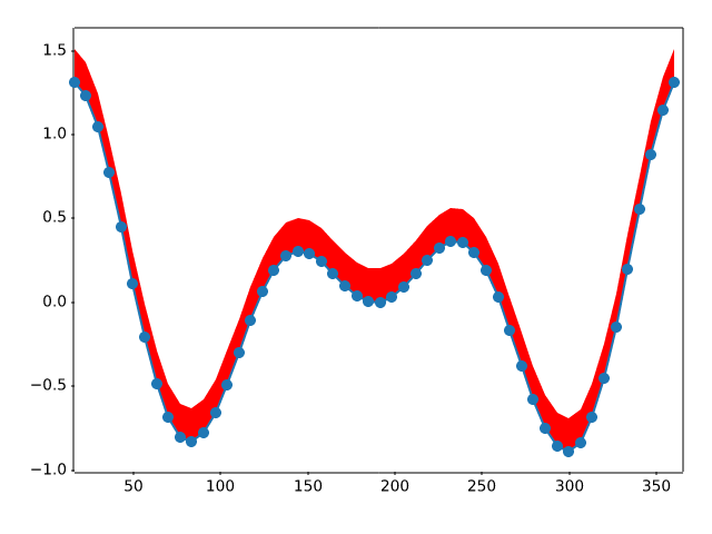
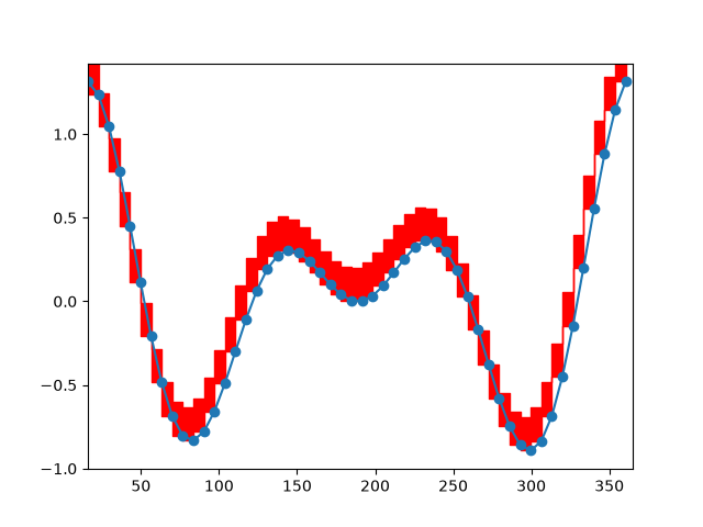
event_handling/timers
======
Source
"""
======
Timers
======

Simple example of using general timer objects. This is used to update
the time placed in the title of the figure.

.. note::
    This example exercises the interactive capabilities of Matplotlib, and this
    will not appear in the static documentation. Please run this code on your
    machine to see the interactivity.

    You can copy and paste individual parts, or download the entire example
    using the link at the bottom of the page.
"""
from datetime import datetime

import matplotlib.pyplot as plt
import numpy as np


def update_title(axes):
    axes.set_title(datetime.now())
    axes.figure.canvas.draw()

fig, ax = plt.subplots()

x = np.linspace(-3, 3)
ax.plot(x, x ** 2)

# Create a new timer object. Set the interval to 100 milliseconds
# (1000 is default) and tell the timer what function should be called.
timer = fig.canvas.new_timer(interval=100)
timer.add_callback(update_title, ax)
timer.start()

# Or could start the timer on first figure draw:
# def start_timer(event):
#     timer.start()
#     fig.canvas.mpl_disconnect(drawid)
# drawid = fig.canvas.mpl_connect('draw_event', start_timer)

plt.show()
event_handling/trifinder_event_demo
====================
Source
"""
====================
Trifinder Event Demo
====================

Example showing the use of a TriFinder object.  As the mouse is moved over the
triangulation, the triangle under the cursor is highlighted and the index of
the triangle is displayed in the plot title.

.. note::
    This example exercises the interactive capabilities of Matplotlib, and this
    will not appear in the static documentation. Please run this code on your
    machine to see the interactivity.

    You can copy and paste individual parts, or download the entire example
    using the link at the bottom of the page.
"""
import matplotlib.pyplot as plt
import numpy as np

from matplotlib.patches import Polygon
from matplotlib.tri import Triangulation


def update_polygon(tri):
    if tri == -1:
        points = [0, 0, 0]
    else:
        points = triang.triangles[tri]
    xs = triang.x[points]
    ys = triang.y[points]
    polygon.set_xy(np.column_stack([xs, ys]))


def on_mouse_move(event):
    if event.inaxes is None:
        tri = -1
    else:
        tri = trifinder(event.xdata, event.ydata)
    update_polygon(tri)
    ax.set_title(f'In triangle {tri}')
    event.canvas.draw()


# Create a Triangulation.
n_angles = 16
n_radii = 5
min_radius = 0.25
radii = np.linspace(min_radius, 0.95, n_radii)
angles = np.linspace(0, 2 * np.pi, n_angles, endpoint=False)
angles = np.repeat(angles[..., np.newaxis], n_radii, axis=1)
angles[:, 1::2] += np.pi / n_angles
x = (radii*np.cos(angles)).flatten()
y = (radii*np.sin(angles)).flatten()
triang = Triangulation(x, y)
triang.set_mask(np.hypot(x[triang.triangles].mean(axis=1),
                         y[triang.triangles].mean(axis=1))
                < min_radius)

# Use the triangulation's default TriFinder object.
trifinder = triang.get_trifinder()

# Setup plot and callbacks.
fig, ax = plt.subplots(subplot_kw={'aspect': 'equal'})
ax.triplot(triang, 'bo-')
polygon = Polygon([[0, 0], [0, 0]], facecolor='y')  # dummy data for (xs, ys)
update_polygon(-1)
ax.add_patch(polygon)
fig.canvas.mpl_connect('motion_notify_event', on_mouse_move)
plt.show()
event_handling/viewlims
========
Source
"""
========
Viewlims
========

Creates two identical panels.  Zooming in on the right panel will show
a rectangle in the first panel, denoting the zoomed region.

.. note::
    This example exercises the interactive capabilities of Matplotlib, and this
    will not appear in the static documentation. Please run this code on your
    machine to see the interactivity.

    You can copy and paste individual parts, or download the entire example
    using the link at the bottom of the page.
"""

import functools

import matplotlib.pyplot as plt
import numpy as np

from matplotlib.patches import Rectangle


# A class that will regenerate a fractal set as we zoom in, so that you
# can actually see the increasing detail.  A box in the left panel will show
# the area to which we are zoomed.
class MandelbrotDisplay:
    def __init__(self, h=500, w=500, niter=50, radius=2., power=2):
        self.height = h
        self.width = w
        self.niter = niter
        self.radius = radius
        self.power = power

    def compute_image(self, xlim, ylim):
        self.x = np.linspace(*xlim, self.width)
        self.y = np.linspace(*ylim, self.height).reshape(-1, 1)
        c = self.x + 1.0j * self.y
        threshold_time = np.zeros((self.height, self.width))
        z = np.zeros(threshold_time.shape, dtype=complex)
        mask = np.ones(threshold_time.shape, dtype=bool)
        for i in range(self.niter):
            z[mask] = z[mask]**self.power + c[mask]
            mask = (np.abs(z) < self.radius)
            threshold_time += mask
        return threshold_time

    def ax_update(self, ax):
        ax.set_autoscale_on(False)  # Otherwise, infinite loop
        # Get the number of points from the number of pixels in the window
        self.width, self.height = ax.patch.get_window_extent().size.round().astype(int)
        # Update the image object with our new data and extent
        ax.images[-1].set(data=self.compute_image(ax.get_xlim(), ax.get_ylim()),
                          extent=(*ax.get_xlim(), *ax.get_ylim()))
        ax.figure.canvas.draw_idle()


md = MandelbrotDisplay()

fig1, (ax_full, ax_zoom) = plt.subplots(1, 2)
ax_zoom.imshow([[0]], origin="lower")  # Empty initial image.
ax_zoom.set_title("Zoom here")

rect = Rectangle(
    [0, 0], 0, 0, facecolor="none", edgecolor="black", linewidth=1.0)
ax_full.add_patch(rect)


def update_rect(rect, ax):  # Let the rectangle track the bounds of the zoom axes.
    xlo, xhi = ax.get_xlim()
    ylo, yhi = ax.get_ylim()
    rect.set_bounds((xlo, ylo, xhi - xlo, yhi - ylo))
    ax.figure.canvas.draw_idle()


# Connect for changing the view limits.
ax_zoom.callbacks.connect("xlim_changed", functools.partial(update_rect, rect))
ax_zoom.callbacks.connect("ylim_changed", functools.partial(update_rect, rect))

ax_zoom.callbacks.connect("xlim_changed", md.ax_update)
ax_zoom.callbacks.connect("ylim_changed", md.ax_update)

# Initialize: trigger image computation by setting view limits; set colormap limits;
# copy image to full view.
ax_zoom.set(xlim=(-2, .5), ylim=(-1.25, 1.25))
im = ax_zoom.images[0]
ax_zoom.images[0].set(clim=(im.get_array().min(), im.get_array().max()))
ax_full.imshow(im.get_array(), extent=im.get_extent(), origin="lower")

plt.show()
event_handling/zoom_window
========================
Source
"""
========================
Zoom modifies other Axes
========================

This example shows how to connect events in one window, for example, a mouse
press, to another figure window.

If you click on a point in the first window, the z and y limits of the second
will be adjusted so that the center of the zoom in the second window will be
the (x, y) coordinates of the clicked point.

Note the diameter of the circles in the scatter are defined in points**2, so
their size is independent of the zoom.

.. note::
    This example exercises the interactive capabilities of Matplotlib, and this
    will not appear in the static documentation. Please run this code on your
    machine to see the interactivity.

    You can copy and paste individual parts, or download the entire example
    using the link at the bottom of the page.
"""

import matplotlib.pyplot as plt
import numpy as np

# Fixing random state for reproducibility
np.random.seed(19680801)

figsrc, axsrc = plt.subplots(figsize=(3.7, 3.7))
figzoom, axzoom = plt.subplots(figsize=(3.7, 3.7))
axsrc.set(xlim=(0, 1), ylim=(0, 1), autoscale_on=False,
          title='Click to zoom')
axzoom.set(xlim=(0.45, 0.55), ylim=(0.4, 0.6), autoscale_on=False,
           title='Zoom window')

x, y, s, c = np.random.rand(4, 200)
s *= 200

axsrc.scatter(x, y, s, c)
axzoom.scatter(x, y, s, c)


def on_press(event):
    if event.button != 1:
        return
    x, y = event.xdata, event.ydata
    axzoom.set_xlim(x - 0.1, x + 0.1)
    axzoom.set_ylim(y - 0.1, y + 0.1)
    figzoom.canvas.draw()

figsrc.canvas.mpl_connect('button_press_event', on_press)
plt.show()
images_contours_and_fields/affine_image
============================
Source
"""
============================
Affine transform of an image
============================


Prepending an affine transformation (`~.transforms.Affine2D`) to the :ref:`data
transform <data-coords>` of an image allows to manipulate the image's shape and
orientation.  This is an example of the concept of :ref:`transform chaining
<transformation-pipeline>`.

The image of the output should have its boundary match the dashed yellow
rectangle.
"""

import matplotlib.pyplot as plt
import numpy as np

import matplotlib.transforms as mtransforms


def get_image():
    delta = 0.25
    x = y = np.arange(-3.0, 3.0, delta)
    X, Y = np.meshgrid(x, y)
    Z1 = np.exp(-X**2 - Y**2)
    Z2 = np.exp(-(X - 1)**2 - (Y - 1)**2)
    Z = (Z1 - Z2)
    return Z


def do_plot(ax, Z, transform):
    im = ax.imshow(Z, interpolation='none',
                   origin='lower',
                   extent=[-2, 4, -3, 2], clip_on=True)

    trans_data = transform + ax.transData
    im.set_transform(trans_data)

    # display intended extent of the image
    x1, x2, y1, y2 = im.get_extent()
    ax.plot([x1, x2, x2, x1, x1], [y1, y1, y2, y2, y1], "y--",
            transform=trans_data)
    ax.set_xlim(-5, 5)
    ax.set_ylim(-4, 4)


# prepare image and figure
fig, ((ax1, ax2), (ax3, ax4)) = plt.subplots(2, 2)
Z = get_image()

# image rotation
do_plot(ax1, Z, mtransforms.Affine2D().rotate_deg(30))

# image skew
do_plot(ax2, Z, mtransforms.Affine2D().skew_deg(30, 15))

# scale and reflection
do_plot(ax3, Z, mtransforms.Affine2D().scale(-1, .5))

# everything and a translation
do_plot(ax4, Z, mtransforms.Affine2D().
        rotate_deg(30).skew_deg(30, 15).scale(-1, .5).translate(.5, -1))

plt.show()


# %%
#
# .. admonition:: References
#
#    The use of the following functions, methods, classes and modules is shown
#    in this example:
#
#    - `matplotlib.axes.Axes.imshow` / `matplotlib.pyplot.imshow`
#    - `matplotlib.transforms.Affine2D`
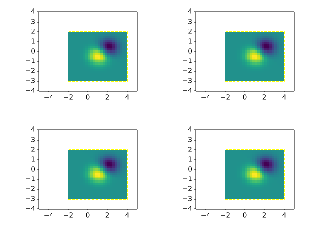
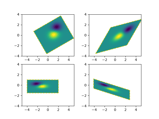
images_contours_and_fields/barb_demo
==========
Source
"""
==========
Wind barbs
==========

Demonstration of wind barb plots.
"""
import matplotlib.pyplot as plt
import numpy as np

x = np.linspace(-5, 5, 5)
X, Y = np.meshgrid(x, x)
U, V = 12 * X, 12 * Y

data = [(-1.5, .5, -6, -6),
        (1, -1, -46, 46),
        (-3, -1, 11, -11),
        (1, 1.5, 80, 80),
        (0.5, 0.25, 25, 15),
        (-1.5, -0.5, -5, 40)]

data = np.array(data, dtype=[('x', np.float32), ('y', np.float32),
                             ('u', np.float32), ('v', np.float32)])

fig1, axs1 = plt.subplots(nrows=2, ncols=2)
# Default parameters, uniform grid
axs1[0, 0].barbs(X, Y, U, V)

# Arbitrary set of vectors, make them longer and change the pivot point
# (point around which they're rotated) to be the middle
axs1[0, 1].barbs(
    data['x'], data['y'], data['u'], data['v'], length=8, pivot='middle')

# Showing colormapping with uniform grid.  Fill the circle for an empty barb,
# don't round the values, and change some of the size parameters
axs1[1, 0].barbs(
    X, Y, U, V, np.sqrt(U ** 2 + V ** 2), fill_empty=True, rounding=False,
    sizes=dict(emptybarb=0.25, spacing=0.2, height=0.3))

# Change colors as well as the increments for parts of the barbs
axs1[1, 1].barbs(data['x'], data['y'], data['u'], data['v'], flagcolor='r',
                 barbcolor=['b', 'g'], flip_barb=True,
                 barb_increments=dict(half=10, full=20, flag=100))

# Masked arrays are also supported
masked_u = np.ma.masked_array(data['u'])
masked_u[4] = 1000  # Bad value that should not be plotted when masked
masked_u[4] = np.ma.masked

# %%
# Identical plot to panel 2 in the first figure, but with the point at
# (0.5, 0.25) missing (masked)
fig2, ax2 = plt.subplots()
ax2.barbs(data['x'], data['y'], masked_u, data['v'], length=8, pivot='middle')

plt.show()

# %%
#
# .. admonition:: References
#
#    The use of the following functions, methods, classes and modules is shown
#    in this example:
#
#    - `matplotlib.axes.Axes.barbs` / `matplotlib.pyplot.barbs`
images_contours_and_fields/barcode_demo
=======
Source
"""
=======
Barcode
=======
This demo shows how to produce a bar code.

The figure size is calculated so that the width in pixels is a multiple of the
number of data points to prevent interpolation artifacts. Additionally, the
``Axes`` is defined to span the whole figure and all ``Axis`` are turned off.

The data itself is rendered with `~.Axes.imshow` using

- ``code.reshape(1, -1)`` to turn the data into a 2D array with one row.
- ``imshow(..., aspect='auto')`` to allow for non-square pixels.
- ``imshow(..., interpolation='nearest')`` to prevent blurred edges. This
  should not happen anyway because we fine-tuned the figure width in pixels,
  but just to be safe.
"""

import matplotlib.pyplot as plt
import numpy as np

code = np.array([
    1, 0, 1, 0, 1, 1, 1, 0, 1, 1, 0, 0, 0, 1, 0, 0, 1, 0, 1, 0, 0, 1, 1, 1,
    0, 0, 0, 1, 0, 1, 1, 0, 0, 0, 0, 1, 0, 1, 0, 0, 1, 1, 0, 0, 1, 0, 1, 0,
    1, 0, 1, 0, 0, 0, 0, 1, 0, 1, 1, 1, 0, 1, 0, 0, 1, 1, 0, 1, 1, 0, 0, 1,
    1, 0, 0, 1, 1, 0, 1, 0, 1, 1, 1, 0, 0, 1, 0, 0, 0, 1, 0, 0, 1, 0, 1])

pixel_per_bar = 4
dpi = 100

fig = plt.figure(figsize=(len(code) * pixel_per_bar / dpi, 2), dpi=dpi)
ax = fig.add_axes((0, 0, 1, 1))  # span the whole figure
ax.set_axis_off()
ax.imshow(code.reshape(1, -1), cmap='binary', aspect='auto',
          interpolation='nearest')
plt.show()

# %%
#
# .. admonition:: References
#
#    The use of the following functions, methods, classes and modules is shown
#    in this example:
#
#    - `matplotlib.axes.Axes.imshow` / `matplotlib.pyplot.imshow`
#    - `matplotlib.figure.Figure.add_axes`
#
# .. tags::
#
#    component: axes
#    plot-type: imshow
#    purpose: fun


images_contours_and_fields/colormap_interactive_adjustment
========================================
Source
"""
========================================
Interactive adjustment of colormap range
========================================

Demonstration of how a colorbar can be used to interactively adjust the
range of colormapping on an image. To use the interactive feature, you must
be in either zoom mode (magnifying glass toolbar button) or
pan mode (4-way arrow toolbar button) and click inside the colorbar.

When zooming, the bounding box of the zoom region defines the new vmin and
vmax of the norm. Zooming using the right mouse button will expand the
vmin and vmax proportionally to the selected region, in the same manner that
one can zoom out on an axis. When panning, the vmin and vmax of the norm are
both shifted according to the direction of movement. The
Home/Back/Forward buttons can also be used to get back to a previous state.

.. redirect-from:: /gallery/userdemo/colormap_interactive_adjustment
"""
import matplotlib.pyplot as plt
import numpy as np

t = np.linspace(0, 2 * np.pi, 1024)
data2d = np.sin(t)[:, np.newaxis] * np.cos(t)[np.newaxis, :]

fig, ax = plt.subplots()
im = ax.imshow(data2d)
ax.set_title('Pan on the colorbar to shift the color mapping\n'
             'Zoom on the colorbar to scale the color mapping')

fig.colorbar(im, ax=ax, label='Interactive colorbar')

plt.show()
images_contours_and_fields/colormap_normalizations
=======================
Source
"""
=======================
Colormap normalizations
=======================

Demonstration of using norm to map colormaps onto data in non-linear ways.

.. redirect-from:: /gallery/userdemo/colormap_normalizations
"""

import matplotlib.pyplot as plt
import numpy as np

import matplotlib.colors as colors

N = 100

# %%
# LogNorm
# -------
# This example data has a low hump with a spike coming out of its center. If plotted
# using a linear colour scale, then only the spike will be visible. To see both hump and
# spike, this requires the z/colour axis on a log scale.
#
# Instead of transforming the data with ``pcolor(log10(Z))``, the color mapping can be
# made logarithmic using a `.LogNorm`.

X, Y = np.mgrid[-3:3:complex(0, N), -2:2:complex(0, N)]
Z1 = np.exp(-X**2 - Y**2)
Z2 = np.exp(-(X * 10)**2 - (Y * 10)**2)
Z = Z1 + 50 * Z2

fig, ax = plt.subplots(2, 1)

pcm = ax[0].pcolor(X, Y, Z, cmap='PuBu_r', shading='nearest')
fig.colorbar(pcm, ax=ax[0], extend='max', label='linear scaling')

pcm = ax[1].pcolor(X, Y, Z, cmap='PuBu_r', shading='nearest',
                   norm=colors.LogNorm(vmin=Z.min(), vmax=Z.max()))
fig.colorbar(pcm, ax=ax[1], extend='max', label='LogNorm')

# %%
# PowerNorm
# ---------
# This example data mixes a power-law trend in X with a rectified sine wave in Y. If
# plotted using a linear colour scale, then the power-law trend in X partially obscures
# the sine wave in Y.
#
# The power law can be removed using a `.PowerNorm`.

X, Y = np.mgrid[0:3:complex(0, N), 0:2:complex(0, N)]
Z = (1 + np.sin(Y * 10)) * X**2

fig, ax = plt.subplots(2, 1)

pcm = ax[0].pcolormesh(X, Y, Z, cmap='PuBu_r', shading='nearest')
fig.colorbar(pcm, ax=ax[0], extend='max', label='linear scaling')

pcm = ax[1].pcolormesh(X, Y, Z, cmap='PuBu_r', shading='nearest',
                       norm=colors.PowerNorm(gamma=0.5))
fig.colorbar(pcm, ax=ax[1], extend='max', label='PowerNorm')

# %%
# SymLogNorm
# ----------
# This example data has two humps, one negative and one positive, The positive hump has
# 5 times the amplitude of the negative. If plotted with a linear colour scale, then
# the detail in the negative hump is obscured.
#
# Here we logarithmically scale the positive and negative data separately with
# `.SymLogNorm`.
#
# Note that colorbar labels do not come out looking very good.

X, Y = np.mgrid[-3:3:complex(0, N), -2:2:complex(0, N)]
Z1 = np.exp(-X**2 - Y**2)
Z2 = np.exp(-(X - 1)**2 - (Y - 1)**2)
Z = (5 * Z1 - Z2) * 2

fig, ax = plt.subplots(2, 1)

pcm = ax[0].pcolormesh(X, Y, Z, cmap='RdBu_r', shading='nearest',
                       vmin=-np.max(Z))
fig.colorbar(pcm, ax=ax[0], extend='both', label='linear scaling')

pcm = ax[1].pcolormesh(X, Y, Z, cmap='RdBu_r', shading='nearest',
                       norm=colors.SymLogNorm(linthresh=0.015,
                                              vmin=-10.0, vmax=10.0, base=10))
fig.colorbar(pcm, ax=ax[1], extend='both', label='SymLogNorm')

# %%
# Custom Norm
# -----------
# Alternatively, the above example data can be scaled with a customized normalization.
# This one normalizes the negative data differently from the positive.


# Example of making your own norm.  Also see matplotlib.colors.
# From Joe Kington: This one gives two different linear ramps:
class MidpointNormalize(colors.Normalize):
    def __init__(self, vmin=None, vmax=None, midpoint=None, clip=False):
        self.midpoint = midpoint
        super().__init__(vmin, vmax, clip)

    def __call__(self, value, clip=None):
        # I'm ignoring masked values and all kinds of edge cases to make a
        # simple example...
        x, y = [self.vmin, self.midpoint, self.vmax], [0, 0.5, 1]
        return np.ma.masked_array(np.interp(value, x, y))


# %%
fig, ax = plt.subplots(2, 1)

pcm = ax[0].pcolormesh(X, Y, Z, cmap='RdBu_r', shading='nearest',
                       vmin=-np.max(Z))
fig.colorbar(pcm, ax=ax[0], extend='both', label='linear scaling')

pcm = ax[1].pcolormesh(X, Y, Z, cmap='RdBu_r', shading='nearest',
                       norm=MidpointNormalize(midpoint=0))
fig.colorbar(pcm, ax=ax[1], extend='both', label='Custom norm')

# %%
# BoundaryNorm
# ------------
# For arbitrarily dividing the color scale, the `.BoundaryNorm` may be used; by
# providing the boundaries for colors, this norm puts the first color in between the
# first pair, the second color between the second pair, etc.

fig, ax = plt.subplots(3, 1, layout='constrained')

pcm = ax[0].pcolormesh(X, Y, Z, cmap='RdBu_r', shading='nearest',
                       vmin=-np.max(Z))
fig.colorbar(pcm, ax=ax[0], extend='both', orientation='vertical',
             label='linear scaling')

# Evenly-spaced bounds gives a contour-like effect.
bounds = np.linspace(-2, 2, 11)
norm = colors.BoundaryNorm(boundaries=bounds, ncolors=256)
pcm = ax[1].pcolormesh(X, Y, Z, cmap='RdBu_r', shading='nearest',
                       norm=norm)
fig.colorbar(pcm, ax=ax[1], extend='both', orientation='vertical',
             label='BoundaryNorm\nlinspace(-2, 2, 11)')

# Unevenly-spaced bounds changes the colormapping.
bounds = np.array([-1, -0.5, 0, 2.5, 5])
norm = colors.BoundaryNorm(boundaries=bounds, ncolors=256)
pcm = ax[2].pcolormesh(X, Y, Z, cmap='RdBu_r', shading='nearest',
                       norm=norm)
fig.colorbar(pcm, ax=ax[2], extend='both', orientation='vertical',
             label='BoundaryNorm\n[-1, -0.5, 0, 2.5, 5]')

plt.show()
images_contours_and_fields/colormap_normalizations_symlognorm
==================================
Source
"""
==================================
Colormap normalizations SymLogNorm
==================================

Demonstration of using norm to map colormaps onto data in non-linear ways.

.. redirect-from:: /gallery/userdemo/colormap_normalization_symlognorm
"""

# %%
# Synthetic dataset consisting of two humps, one negative and one positive,
# the positive with 8-times the amplitude.
# Linearly, the negative hump is almost invisible,
# and it is very difficult to see any detail of its profile.
# With the logarithmic scaling applied to both positive and negative values,
# it is much easier to see the shape of each hump.
#
# See `~.colors.SymLogNorm`.

import matplotlib.pyplot as plt
import numpy as np

import matplotlib.colors as colors


def rbf(x, y):
    return 1.0 / (1 + 5 * ((x ** 2) + (y ** 2)))

N = 200
gain = 8
X, Y = np.mgrid[-3:3:complex(0, N), -2:2:complex(0, N)]
Z1 = rbf(X + 0.5, Y + 0.5)
Z2 = rbf(X - 0.5, Y - 0.5)
Z = gain * Z1 - Z2

shadeopts = {'cmap': 'PRGn', 'shading': 'gouraud'}
colormap = 'PRGn'
lnrwidth = 0.5

fig, ax = plt.subplots(2, 1, sharex=True, sharey=True)

pcm = ax[0].pcolormesh(X, Y, Z,
                       norm=colors.SymLogNorm(linthresh=lnrwidth, linscale=1,
                                              vmin=-gain, vmax=gain, base=10),
                       **shadeopts)
fig.colorbar(pcm, ax=ax[0], extend='both')
ax[0].text(-2.5, 1.5, 'symlog')

pcm = ax[1].pcolormesh(X, Y, Z, vmin=-gain, vmax=gain,
                       **shadeopts)
fig.colorbar(pcm, ax=ax[1], extend='both')
ax[1].text(-2.5, 1.5, 'linear')


# %%
# In order to find the best visualization for any particular dataset,
# it may be necessary to experiment with multiple different color scales.
# As well as the `~.colors.SymLogNorm` scaling, there is also
# the option of using `~.colors.AsinhNorm` (experimental), which has a smoother
# transition between the linear and logarithmic regions of the transformation
# applied to the data values, "Z".
# In the plots below, it may be possible to see contour-like artifacts
# around each hump despite there being no sharp features
# in the dataset itself. The ``asinh`` scaling shows a smoother shading
# of each hump.

fig, ax = plt.subplots(2, 1, sharex=True, sharey=True)

pcm = ax[0].pcolormesh(X, Y, Z,
                       norm=colors.SymLogNorm(linthresh=lnrwidth, linscale=1,
                                              vmin=-gain, vmax=gain, base=10),
                       **shadeopts)
fig.colorbar(pcm, ax=ax[0], extend='both')
ax[0].text(-2.5, 1.5, 'symlog')

pcm = ax[1].pcolormesh(X, Y, Z,
                       norm=colors.AsinhNorm(linear_width=lnrwidth,
                                             vmin=-gain, vmax=gain),
                       **shadeopts)
fig.colorbar(pcm, ax=ax[1], extend='both')
ax[1].text(-2.5, 1.5, 'asinh')


plt.show()
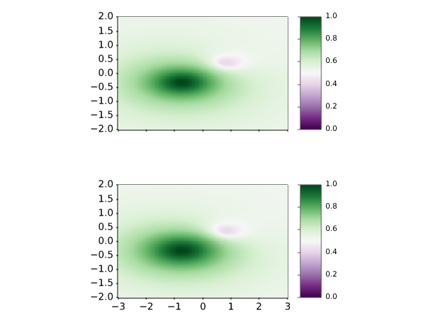
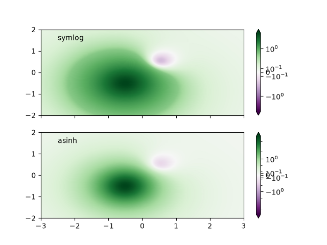
images_contours_and_fields/contour_corner_mask
===================
Source
"""
===================
Contour corner mask
===================

Illustrate the difference between ``corner_mask=False`` and
``corner_mask=True`` for masked contour plots.  The default is controlled by
:rc:`contour.corner_mask`.
"""

import matplotlib.pyplot as plt
import numpy as np

# Data to plot.
x, y = np.meshgrid(np.arange(7), np.arange(10))
z = np.sin(0.5 * x) * np.cos(0.52 * y)

# Mask various z values.
mask = np.zeros_like(z, dtype=bool)
mask[2, 3:5] = True
mask[3:5, 4] = True
mask[7, 2] = True
mask[5, 0] = True
mask[0, 6] = True
z = np.ma.array(z, mask=mask)

corner_masks = [False, True]
fig, axs = plt.subplots(ncols=2)
for ax, corner_mask in zip(axs, corner_masks):
    cs = ax.contourf(x, y, z, corner_mask=corner_mask)
    ax.contour(cs, colors='k')
    ax.set_title(f'{corner_mask=}')

    # Plot grid.
    ax.grid(c='k', ls='-', alpha=0.3)

    # Indicate masked points with red circles.
    ax.plot(np.ma.array(x, mask=~mask), y, 'ro')

plt.show()

# %%
#
# .. admonition:: References
#
#    The use of the following functions, methods, classes and modules is shown
#    in this example:
#
#    - `matplotlib.axes.Axes.contour` / `matplotlib.pyplot.contour`
#    - `matplotlib.axes.Axes.contourf` / `matplotlib.pyplot.contourf`
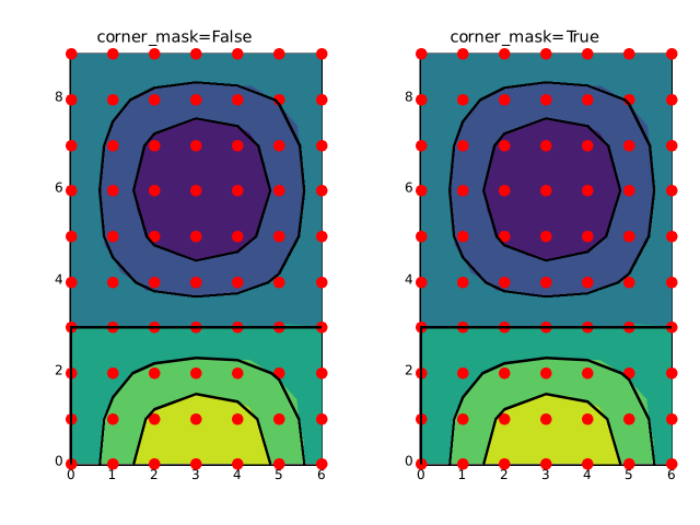
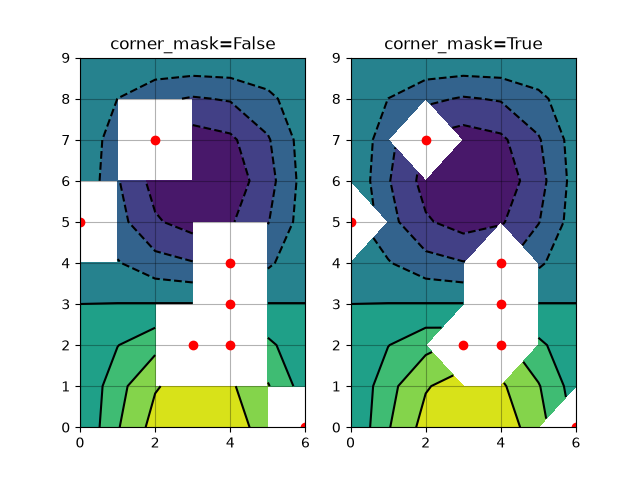
images_contours_and_fields/contour_demo
============
Source
"""
============
Contour Demo
============

Illustrate simple contour plotting, contours on an image with
a colorbar for the contours, and labelled contours.

See also the :doc:`contour image example
</gallery/images_contours_and_fields/contour_image>`.
"""

import matplotlib.pyplot as plt
import numpy as np

delta = 0.025
x = np.arange(-3.0, 3.0, delta)
y = np.arange(-2.0, 2.0, delta)
X, Y = np.meshgrid(x, y)
Z1 = np.exp(-X**2 - Y**2)
Z2 = np.exp(-(X - 1)**2 - (Y - 1)**2)
Z = (Z1 - Z2) * 2

# %%
# Create a simple contour plot with labels using default colors.  The inline
# argument to clabel will control whether the labels are draw over the line
# segments of the contour, removing the lines beneath the label.

fig, ax = plt.subplots()
CS = ax.contour(X, Y, Z)
ax.clabel(CS, fontsize=10)
ax.set_title('Simplest default with labels')

# %%
# Contour labels can be placed manually by providing list of positions (in data
# coordinate).  See :doc:`/gallery/event_handling/ginput_manual_clabel_sgskip`
# for interactive placement.

fig, ax = plt.subplots()
CS = ax.contour(X, Y, Z)
manual_locations = [
    (-1, -1.4), (-0.62, -0.7), (-2, 0.5), (1.7, 1.2), (2.0, 1.4), (2.4, 1.7)]
ax.clabel(CS, fontsize=10, manual=manual_locations)
ax.set_title('labels at selected locations')

# %%
# You can force all the contours to be the same color.

fig, ax = plt.subplots()
CS = ax.contour(X, Y, Z, 6, colors='k')  # Negative contours default to dashed.
ax.clabel(CS, fontsize=9)
ax.set_title('Single color - negative contours dashed')

# %%
# You can set negative contours to be solid instead of dashed:

plt.rcParams['contour.negative_linestyle'] = 'solid'
fig, ax = plt.subplots()
CS = ax.contour(X, Y, Z, 6, colors='k')  # Negative contours default to dashed.
ax.clabel(CS, fontsize=9)
ax.set_title('Single color - negative contours solid')

# %%
# And you can manually specify the colors of the contour

fig, ax = plt.subplots()
CS = ax.contour(X, Y, Z, 6,
                linewidths=np.arange(.5, 4, .5),
                colors=('r', 'green', 'blue', (1, 1, 0), '#afeeee', '0.5'),
                )
ax.clabel(CS, fontsize=9)
ax.set_title('Crazy lines')

# %%
# Or you can use a colormap to specify the colors; the default
# colormap will be used for the contour lines

fig, ax = plt.subplots()
im = ax.imshow(Z, interpolation='bilinear', origin='lower',
               cmap="gray", extent=(-3, 3, -2, 2))
levels = np.arange(-1.2, 1.6, 0.2)
CS = ax.contour(Z, levels, origin='lower', cmap='flag', extend='both',
                linewidths=2, extent=(-3, 3, -2, 2))

# Thicken the zero contour.
lws = np.resize(CS.get_linewidth(), len(levels))
lws[6] = 4
CS.set_linewidth(lws)

ax.clabel(CS, levels[1::2],  # label every second level
          fmt='%1.1f', fontsize=14)

# make a colorbar for the contour lines
CB = fig.colorbar(CS, shrink=0.8)

ax.set_title('Lines with colorbar')

# We can still add a colorbar for the image, too.
CBI = fig.colorbar(im, orientation='horizontal', shrink=0.8)

# This makes the original colorbar look a bit out of place,
# so let's improve its position.

l, b, w, h = ax.get_position().bounds
ll, bb, ww, hh = CB.ax.get_position().bounds
CB.ax.set_position([ll, b + 0.1*h, ww, h*0.8])

plt.show()

# %%
#
# .. admonition:: References
#
#    The use of the following functions, methods, classes and modules is shown
#    in this example:
#
#    - `matplotlib.axes.Axes.contour` / `matplotlib.pyplot.contour`
#    - `matplotlib.figure.Figure.colorbar` / `matplotlib.pyplot.colorbar`
#    - `matplotlib.axes.Axes.clabel` / `matplotlib.pyplot.clabel`
#    - `matplotlib.axes.Axes.get_position`
#    - `matplotlib.axes.Axes.set_position`
NotImplementedError: manual clabel placement is not supported
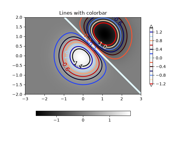
images_contours_and_fields/contour_image
=============
Source
"""
=============
Contour image
=============

Test combinations of contouring, filled contouring, and image plotting.
For contour labelling, see also the :doc:`contour demo example
</gallery/images_contours_and_fields/contour_demo>`.

The emphasis in this demo is on showing how to make contours register
correctly on images, and on how to get both of them oriented as desired.
In particular, note the usage of the :ref:`"origin" and "extent"
<imshow_extent>` keyword arguments to imshow and
contour.
"""
import matplotlib.pyplot as plt
import numpy as np

from matplotlib import cm

# Default delta is large because that makes it fast, and it illustrates
# the correct registration between image and contours.
delta = 0.5

extent = (-3, 4, -4, 3)

x = np.arange(-3.0, 4.001, delta)
y = np.arange(-4.0, 3.001, delta)
X, Y = np.meshgrid(x, y)
Z1 = np.exp(-X**2 - Y**2)
Z2 = np.exp(-(X - 1)**2 - (Y - 1)**2)
Z = (Z1 - Z2) * 2

# Boost the upper limit to avoid truncation errors.
levels = np.arange(-2.0, 1.601, 0.4)

norm = cm.colors.Normalize(vmax=abs(Z).max(), vmin=-abs(Z).max())
cmap = plt.colormaps["PRGn"]

fig, _axs = plt.subplots(nrows=2, ncols=2)
fig.subplots_adjust(hspace=0.3)
axs = _axs.flatten()

cset1 = axs[0].contourf(X, Y, Z, levels, norm=norm,
                        cmap=cmap.resampled(len(levels) - 1))
# It is not necessary, but for the colormap, we need only the
# number of levels minus 1.  To avoid discretization error, use
# either this number or a large number such as the default (256).

# If we want lines as well as filled regions, we need to call
# contour separately; don't try to change the edgecolor or edgewidth
# of the polygons in the collections returned by contourf.
# Use levels output from previous call to guarantee they are the same.

cset2 = axs[0].contour(X, Y, Z, cset1.levels, colors='k')

# We don't really need dashed contour lines to indicate negative
# regions, so let's turn them off.
cset2.set_linestyle('solid')

# It is easier here to make a separate call to contour than
# to set up an array of colors and linewidths.
# We are making a thick green line as a zero contour.
# Specify the zero level as a tuple with only 0 in it.

cset3 = axs[0].contour(X, Y, Z, (0,), colors='g', linewidths=2)
axs[0].set_title('Filled contours')
fig.colorbar(cset1, ax=axs[0])


axs[1].imshow(Z, extent=extent, cmap=cmap, norm=norm)
axs[1].contour(Z, levels, colors='k', origin='upper', extent=extent)
axs[1].set_title("Image, origin 'upper'")

axs[2].imshow(Z, origin='lower', extent=extent, cmap=cmap, norm=norm)
axs[2].contour(Z, levels, colors='k', origin='lower', extent=extent)
axs[2].set_title("Image, origin 'lower'")

# We will use the interpolation "nearest" here to show the actual
# image pixels.
# Note that the contour lines don't extend to the edge of the box.
# This is intentional. The Z values are defined at the center of each
# image pixel (each color block on the following subplot), so the
# domain that is contoured does not extend beyond these pixel centers.
im = axs[3].imshow(Z, interpolation='nearest', extent=extent,
                   cmap=cmap, norm=norm)
axs[3].contour(Z, levels, colors='k', origin='image', extent=extent)
ylim = axs[3].get_ylim()
axs[3].set_ylim(ylim[::-1])
axs[3].set_title("Origin from rc, reversed y-axis")
fig.colorbar(im, ax=axs[3])

fig.tight_layout()
plt.show()


# %%
#
# .. admonition:: References
#
#    The use of the following functions, methods, classes and modules is shown
#    in this example:
#
#    - `matplotlib.axes.Axes.contour` / `matplotlib.pyplot.contour`
#    - `matplotlib.axes.Axes.imshow` / `matplotlib.pyplot.imshow`
#    - `matplotlib.figure.Figure.colorbar` / `matplotlib.pyplot.colorbar`
#    - `matplotlib.colors.Normalize`
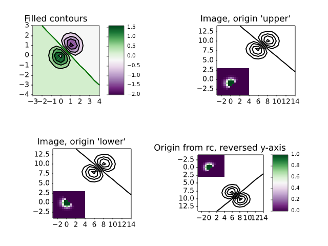
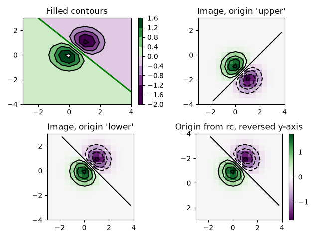
images_contours_and_fields/contour_label_demo
==================
Source
"""
==================
Contour Label Demo
==================

Illustrate some of the more advanced things that one can do with
contour labels.

See also the :doc:`contour demo example
</gallery/images_contours_and_fields/contour_demo>`.
"""

import matplotlib.pyplot as plt
import numpy as np

import matplotlib.ticker as ticker

# %%
# Define our surface

delta = 0.025
x = np.arange(-3.0, 3.0, delta)
y = np.arange(-2.0, 2.0, delta)
X, Y = np.meshgrid(x, y)
Z1 = np.exp(-X**2 - Y**2)
Z2 = np.exp(-(X - 1)**2 - (Y - 1)**2)
Z = (Z1 - Z2) * 2

# %%
# Make contour labels with custom level formatters


# This custom formatter removes trailing zeros, e.g. "1.0" becomes "1", and
# then adds a percent sign.
def fmt(x):
    s = f"{x:.1f}"
    if s.endswith("0"):
        s = f"{x:.0f}"
    return rf"{s} \%" if plt.rcParams["text.usetex"] else f"{s} %"


# Basic contour plot
fig, ax = plt.subplots()
CS = ax.contour(X, Y, Z)

ax.clabel(CS, CS.levels, fmt=fmt, fontsize=10)

# %%
# Label contours with arbitrary strings using a dictionary

fig1, ax1 = plt.subplots()

# Basic contour plot
CS1 = ax1.contour(X, Y, Z)

fmt = {}
strs = ['first', 'second', 'third', 'fourth', 'fifth', 'sixth', 'seventh']
for l, s in zip(CS1.levels, strs):
    fmt[l] = s

# Label every other level using strings
ax1.clabel(CS1, CS1.levels[::2], fmt=fmt, fontsize=10)

# %%
# Use a Formatter

fig2, ax2 = plt.subplots()

CS2 = ax2.contour(X, Y, 100**Z, locator=plt.LogLocator())
fmt = ticker.LogFormatterMathtext()
fmt.create_dummy_axis()
ax2.clabel(CS2, CS2.levels, fmt=fmt)
ax2.set_title("$100^Z$")

plt.show()

# %%
#
# .. admonition:: References
#
#    The use of the following functions, methods, classes and modules is shown
#    in this example:
#
#    - `matplotlib.axes.Axes.contour` / `matplotlib.pyplot.contour`
#    - `matplotlib.axes.Axes.clabel` / `matplotlib.pyplot.clabel`
#    - `matplotlib.ticker.LogFormatterMathtext`
#    - `matplotlib.ticker.TickHelper.create_dummy_axis`
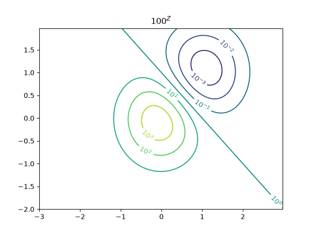
images_contours_and_fields/contourf_demo
=============
Source
"""
=============
Contourf demo
=============

How to use the `.axes.Axes.contourf` method to create filled contour plots.
"""
import matplotlib.pyplot as plt
import numpy as np

delta = 0.025

x = y = np.arange(-3.0, 3.01, delta)
X, Y = np.meshgrid(x, y)
Z1 = np.exp(-X**2 - Y**2)
Z2 = np.exp(-(X - 1)**2 - (Y - 1)**2)
Z = (Z1 - Z2) * 2

nr, nc = Z.shape

# put NaNs in one corner:
Z[-nr // 6:, -nc // 6:] = np.nan
# contourf will convert these to masked


Z = np.ma.array(Z)
# mask another corner:
Z[:nr // 6, :nc // 6] = np.ma.masked

# mask a circle in the middle:
interior = np.sqrt(X**2 + Y**2) < 0.5
Z[interior] = np.ma.masked

# %%
# Automatic contour levels
# ------------------------
# We are using automatic selection of contour levels; this is usually not such
# a good idea, because they don't occur on nice boundaries, but we do it here
# for purposes of illustration.

fig1, ax2 = plt.subplots(layout='constrained')
CS = ax2.contourf(X, Y, Z, 10, cmap="bone")

# Note that in the following, we explicitly pass in a subset of the contour
# levels used for the filled contours.  Alternatively, we could pass in
# additional levels to provide extra resolution, or leave out the *levels*
# keyword argument to use all of the original levels.

CS2 = ax2.contour(CS, levels=CS.levels[::2], colors='r')

ax2.set_title('Nonsense (3 masked regions)')
ax2.set_xlabel('word length anomaly')
ax2.set_ylabel('sentence length anomaly')

# Make a colorbar for the ContourSet returned by the contourf call.
cbar = fig1.colorbar(CS)
cbar.ax.set_ylabel('verbosity coefficient')
# Add the contour line levels to the colorbar
cbar.add_lines(CS2)

# %%
# Explicit contour levels
# -----------------------
# Now make a contour plot with the levels specified, and with the colormap
# generated automatically from a list of colors.

fig2, ax2 = plt.subplots(layout='constrained')
levels = [-1.5, -1, -0.5, 0, 0.5, 1]
CS3 = ax2.contourf(X, Y, Z, levels, colors=('r', 'g', 'b'), extend='both')
# Our data range extends outside the range of levels; make
# data below the lowest contour level yellow, and above the
# highest level cyan:
CS3.cmap.set_under('yellow')
CS3.cmap.set_over('cyan')

CS4 = ax2.contour(X, Y, Z, levels, colors=('k',), linewidths=(3,))
ax2.set_title('Listed colors (3 masked regions)')
ax2.clabel(CS4, fmt='%2.1f', colors='w', fontsize=14)

# Notice that the colorbar gets all the information it
# needs from the ContourSet object, CS3.
fig2.colorbar(CS3)

# %%
# Extension settings
# ------------------
# Illustrate all 4 possible "extend" settings:
extends = ["neither", "both", "min", "max"]
cmap = plt.colormaps["winter"].with_extremes(under="magenta", over="yellow")
# Note: contouring simply excludes masked or nan regions, so
# instead of using the "bad" colormap value for them, it draws
# nothing at all in them.  Therefore, the following would have
# no effect:
# cmap.set_bad("red")

fig, axs = plt.subplots(2, 2, layout="constrained")

for ax, extend in zip(axs.flat, extends):
    cs = ax.contourf(X, Y, Z, levels, cmap=cmap, extend=extend)
    fig.colorbar(cs, ax=ax, shrink=0.9)
    ax.set_title("extend = %s" % extend)
    ax.locator_params(nbins=4)

plt.show()

# %%
# Orient contour plots using the origin keyword
# ---------------------------------------------
# This code demonstrates orienting contour plot data using the "origin" keyword

x = np.arange(1, 10)
y = x.reshape(-1, 1)
h = x * y

fig, (ax1, ax2) = plt.subplots(ncols=2)

ax1.set_title("origin='upper'")
ax2.set_title("origin='lower'")
ax1.contourf(h, levels=np.arange(5, 70, 5), extend='both', origin="upper")
ax2.contourf(h, levels=np.arange(5, 70, 5), extend='both', origin="lower")

plt.show()

# %%
#
# .. admonition:: References
#
#    The use of the following functions, methods, classes and modules is shown
#    in this example:
#
#    - `matplotlib.axes.Axes.contour` / `matplotlib.pyplot.contour`
#    - `matplotlib.axes.Axes.contourf` / `matplotlib.pyplot.contourf`
#    - `matplotlib.axes.Axes.clabel` / `matplotlib.pyplot.clabel`
#    - `matplotlib.figure.Figure.colorbar` / `matplotlib.pyplot.colorbar`
#    - `matplotlib.colors.Colormap`
#    - `matplotlib.colors.Colormap.set_bad`
#    - `matplotlib.colors.Colormap.set_under`
#    - `matplotlib.colors.Colormap.set_over`
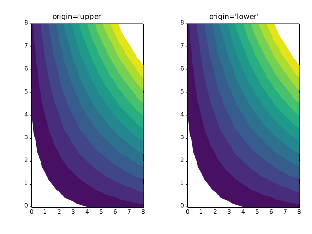
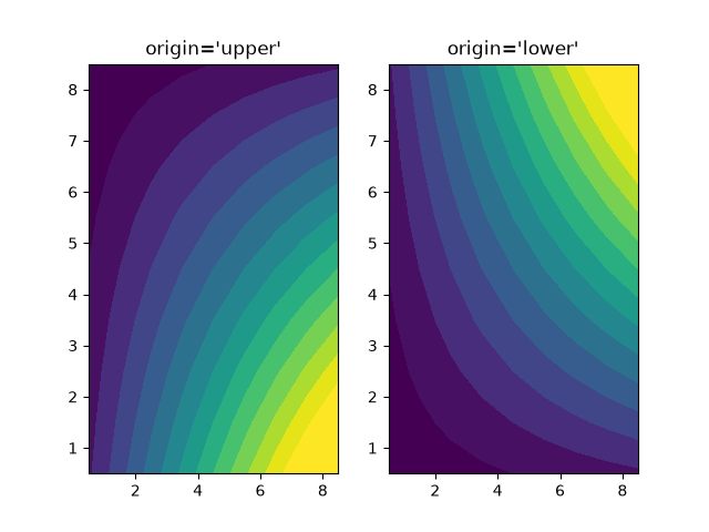
images_contours_and_fields/contourf_hatching
=================
Source
"""
=================
Contourf hatching
=================

Demo filled contour plots with hatched patterns.
"""
import matplotlib.pyplot as plt
import numpy as np

# invent some numbers, turning the x and y arrays into simple
# 2d arrays, which make combining them together easier.
x = np.linspace(-3, 5, 150).reshape(1, -1)
y = np.linspace(-3, 5, 120).reshape(-1, 1)
z = np.cos(x) + np.sin(y)

# we no longer need x and y to be 2 dimensional, so flatten them.
x, y = x.flatten(), y.flatten()

# %%
# Plot 1: the simplest hatched plot with a colorbar

fig1, ax1 = plt.subplots()
cs = ax1.contourf(x, y, z, hatches=['-', '/', '\\', '//'],
                  cmap='gray', extend='both', alpha=0.5)
fig1.colorbar(cs)

# %%
# Plot 2: a plot of hatches without color with a legend

fig2, ax2 = plt.subplots()
n_levels = 6
ax2.contour(x, y, z, n_levels, colors='black', linestyles='-')
cs = ax2.contourf(x, y, z, n_levels, colors='none',
                  hatches=['.', '/', '\\', None, r'\\', '*'],
                  extend='lower')

# create a legend for the contour set
artists, labels = cs.legend_elements(str_format='{:2.1f}'.format)
ax2.legend(artists, labels, handleheight=2, framealpha=1)
plt.show()

# %%
#
# .. admonition:: References
#
#    The use of the following functions, methods, classes and modules is shown
#    in this example:
#
#    - `matplotlib.axes.Axes.contour` / `matplotlib.pyplot.contour`
#    - `matplotlib.axes.Axes.contourf` / `matplotlib.pyplot.contourf`
#    - `matplotlib.figure.Figure.colorbar` / `matplotlib.pyplot.colorbar`
#    - `matplotlib.axes.Axes.legend` / `matplotlib.pyplot.legend`
#    - `matplotlib.contour.ContourSet`
#    - `matplotlib.contour.ContourSet.legend_elements`
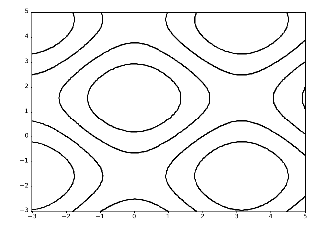
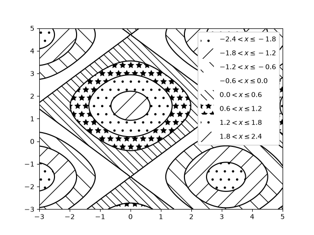
images_contours_and_fields/contourf_log
============================
Source
"""
============================
Contourf and log color scale
============================

Demonstrate use of a log color scale in contourf
"""

import matplotlib.pyplot as plt
import numpy as np
from numpy import ma

from matplotlib import ticker

N = 100
x = np.linspace(-3.0, 3.0, N)
y = np.linspace(-2.0, 2.0, N)

X, Y = np.meshgrid(x, y)

# A low hump with a spike coming out.
# Needs to have z/colour axis on a log scale, so we see both hump and spike.
# A linear scale only shows the spike.
Z1 = np.exp(-X**2 - Y**2)
Z2 = np.exp(-(X * 10)**2 - (Y * 10)**2)
z = Z1 + 50 * Z2

# Put in some negative values (lower left corner) to cause trouble with logs:
z[:5, :5] = -1

# The following is not strictly essential, but it will eliminate
# a warning.  Comment it out to see the warning.
z = ma.masked_where(z <= 0, z)


# Automatic selection of levels works; setting the
# log locator tells contourf to use a log scale:
fig, ax = plt.subplots()
cs = ax.contourf(X, Y, z, locator=ticker.LogLocator(), cmap="PuBu_r")

# Alternatively, you can manually set the levels
# and the norm:
# lev_exp = np.arange(np.floor(np.log10(z.min())-1),
#                    np.ceil(np.log10(z.max())+1))
# levs = np.power(10, lev_exp)
# cs = ax.contourf(X, Y, z, levs, norm=colors.LogNorm())

cbar = fig.colorbar(cs)

plt.show()

# %%
#
# .. admonition:: References
#
#    The use of the following functions, methods, classes and modules is shown
#    in this example:
#
#    - `matplotlib.axes.Axes.contourf` / `matplotlib.pyplot.contourf`
#    - `matplotlib.figure.Figure.colorbar` / `matplotlib.pyplot.colorbar`
#    - `matplotlib.axes.Axes.legend` / `matplotlib.pyplot.legend`
#    - `matplotlib.ticker.LogLocator`
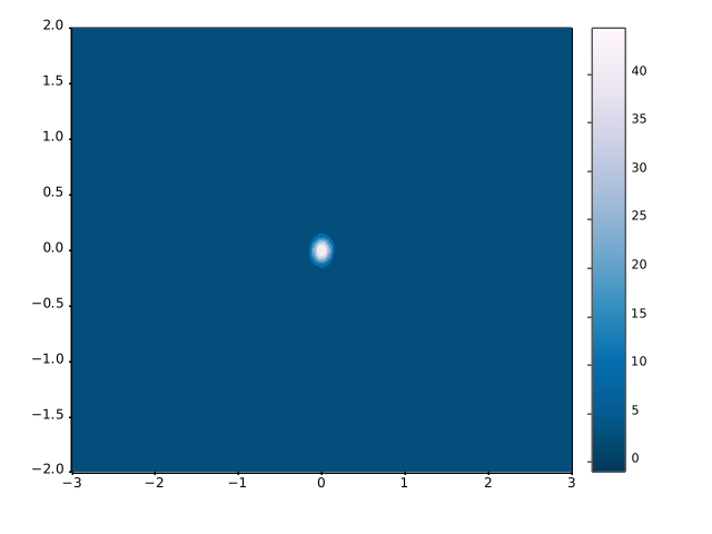
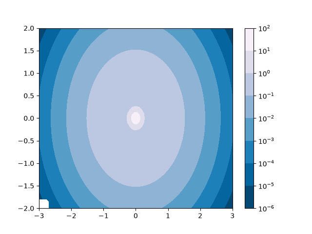
images_contours_and_fields/contours_in_optimization_demo
==============================================
Source
"""
==============================================
Contouring the solution space of optimizations
==============================================

Contour plotting is particularly handy when illustrating the solution
space of optimization problems.  Not only can `.axes.Axes.contour` be
used to represent the topography of the objective function, it can be
used to generate boundary curves of the constraint functions.  The
constraint lines can be drawn with
`~matplotlib.patheffects.TickedStroke` to distinguish the valid and
invalid sides of the constraint boundaries.

`.axes.Axes.contour` generates curves with larger values to the left
of the contour.  The angle parameter is measured zero ahead with
increasing values to the left.  Consequently, when using
`~matplotlib.patheffects.TickedStroke` to illustrate a constraint in
a typical optimization problem, the angle should be set between
zero and 180 degrees.
"""

import matplotlib.pyplot as plt
import numpy as np

from matplotlib import patheffects

fig, ax = plt.subplots(figsize=(6, 6))

nx = 101
ny = 105

# Set up survey vectors
xvec = np.linspace(0.001, 4.0, nx)
yvec = np.linspace(0.001, 4.0, ny)

# Set up survey matrices.  Design disk loading and gear ratio.
x1, x2 = np.meshgrid(xvec, yvec)

# Evaluate some stuff to plot
obj = x1**2 + x2**2 - 2*x1 - 2*x2 + 2
g1 = -(3*x1 + x2 - 5.5)
g2 = -(x1 + 2*x2 - 4.5)
g3 = 0.8 + x1**-3 - x2

cntr = ax.contour(x1, x2, obj, [0.01, 0.1, 0.5, 1, 2, 4, 8, 16],
                  colors='black')
ax.clabel(cntr, fmt="%2.1f", use_clabeltext=True)

cg1 = ax.contour(x1, x2, g1, [0], colors='sandybrown')
cg1.set(path_effects=[patheffects.withTickedStroke(angle=135)])

cg2 = ax.contour(x1, x2, g2, [0], colors='orangered')
cg2.set(path_effects=[patheffects.withTickedStroke(angle=60, length=2)])

cg3 = ax.contour(x1, x2, g3, [0], colors='mediumblue')
cg3.set(path_effects=[patheffects.withTickedStroke(spacing=7)])

ax.set_xlim(0, 4)
ax.set_ylim(0, 4)

plt.show()
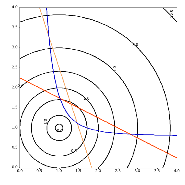
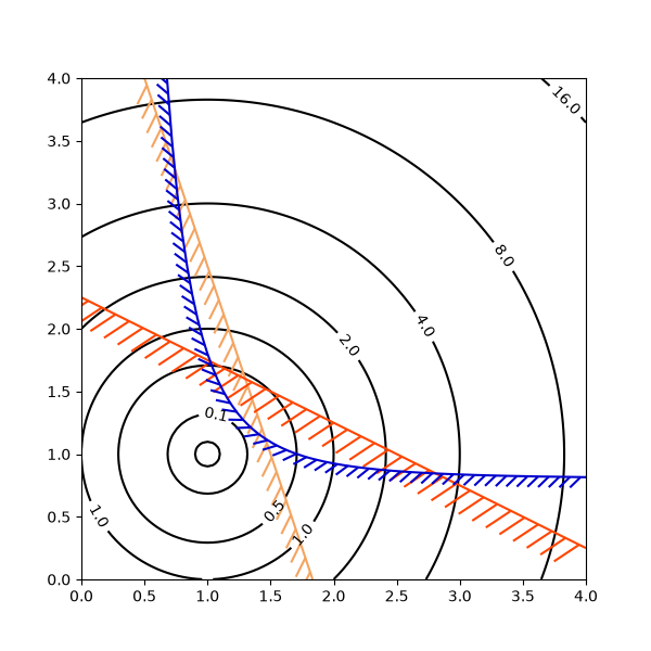
images_contours_and_fields/demo_bboximage
==============
Source
"""
==============
BboxImage Demo
==============

A `~matplotlib.image.BboxImage` can be used to position an image according to
a bounding box. This demo shows how to show an image inside a `.text.Text`'s
bounding box as well as how to manually create a bounding box for the image.
"""

import matplotlib.pyplot as plt
import numpy as np

from matplotlib.image import BboxImage
from matplotlib.transforms import Bbox, TransformedBbox

fig, (ax1, ax2) = plt.subplots(ncols=2)

# ----------------------------
# Create a BboxImage with Text
# ----------------------------
txt = ax1.text(0.5, 0.5, "test", size=30, ha="center", color="w")
ax1.add_artist(
    BboxImage(txt.get_window_extent, data=np.arange(256).reshape((1, -1))))

# ------------------------------------
# Create a BboxImage for each colormap
# ------------------------------------
# List of all colormaps; skip reversed colormaps.
cmap_names = sorted(m for m in plt.colormaps if not m.endswith("_r"))

ncol = 2
nrow = len(cmap_names) // ncol + 1

xpad_fraction = 0.3
dx = 1 / (ncol + xpad_fraction * (ncol - 1))

ypad_fraction = 0.3
dy = 1 / (nrow + ypad_fraction * (nrow - 1))

for i, cmap_name in enumerate(cmap_names):
    ix, iy = divmod(i, nrow)
    bbox0 = Bbox.from_bounds(ix*dx*(1+xpad_fraction),
                             1 - iy*dy*(1+ypad_fraction) - dy,
                             dx, dy)
    bbox = TransformedBbox(bbox0, ax2.transAxes)
    ax2.add_artist(
        BboxImage(bbox, cmap=cmap_name, data=np.arange(256).reshape((1, -1))))

plt.show()

# %%
#
# .. admonition:: References
#
#    The use of the following functions, methods, classes and modules is shown
#    in this example:
#
#    - `matplotlib.image.BboxImage`
#    - `matplotlib.transforms.Bbox`
#    - `matplotlib.transforms.TransformedBbox`
#    - `matplotlib.text.Text`
images_contours_and_fields/figimage_demo
=============
Source
"""
=============
Figimage Demo
=============

This illustrates placing images directly in the figure, with no Axes objects.

"""
import matplotlib.pyplot as plt
import numpy as np

fig = plt.figure()
Z = np.arange(10000).reshape((100, 100))
Z[:, 50:] = 1

im1 = fig.figimage(Z, xo=50, yo=0, origin='lower')
im2 = fig.figimage(Z, xo=100, yo=100, alpha=.8, origin='lower')

plt.show()

# %%
#
# .. admonition:: References
#
#    The use of the following functions, methods, classes and modules is shown
#    in this example:
#
#    - `matplotlib.figure.Figure`
#    - `matplotlib.figure.Figure.figimage` / `matplotlib.pyplot.figimage`


images_contours_and_fields/image_annotated_heatmap
=================
Source
"""
=================
Annotated heatmap
=================

It is often desirable to show data which depends on two independent
variables as a color coded image plot. This is often referred to as a
heatmap. If the data is categorical, this would be called a categorical
heatmap.

Matplotlib's `~matplotlib.axes.Axes.imshow` function makes
production of such plots particularly easy.

The following examples show how to create a heatmap with annotations.
We will start with an easy example and expand it to be usable as a
universal function.
"""


# %%
#
# A simple categorical heatmap
# ----------------------------
#
# We may start by defining some data. What we need is a 2D list or array
# which defines the data to color code. We then also need two lists or arrays
# of categories; of course the number of elements in those lists
# need to match the data along the respective axes.
# The heatmap itself is an `~matplotlib.axes.Axes.imshow` plot
# with the labels set to the categories we have.
# Note that it is important to set both, the tick locations
# (`~matplotlib.axes.Axes.set_xticks`) as well as the
# tick labels (`~matplotlib.axes.Axes.set_xticklabels`),
# otherwise they would become out of sync. The locations are just
# the ascending integer numbers, while the ticklabels are the labels to show.
# Finally, we can label the data itself by creating a `~matplotlib.text.Text`
# within each cell showing the value of that cell.


import matplotlib.pyplot as plt
import numpy as np

import matplotlib
import matplotlib as mpl

# sphinx_gallery_thumbnail_number = 2

vegetables = ["cucumber", "tomato", "lettuce", "asparagus",
              "potato", "wheat", "barley"]
farmers = ["Farmer Joe", "Upland Bros.", "Smith Gardening",
           "Agrifun", "Organiculture", "BioGoods Ltd.", "Cornylee Corp."]

harvest = np.array([[0.8, 2.4, 2.5, 3.9, 0.0, 4.0, 0.0],
                    [2.4, 0.0, 4.0, 1.0, 2.7, 0.0, 0.0],
                    [1.1, 2.4, 0.8, 4.3, 1.9, 4.4, 0.0],
                    [0.6, 0.0, 0.3, 0.0, 3.1, 0.0, 0.0],
                    [0.7, 1.7, 0.6, 2.6, 2.2, 6.2, 0.0],
                    [1.3, 1.2, 0.0, 0.0, 0.0, 3.2, 5.1],
                    [0.1, 2.0, 0.0, 1.4, 0.0, 1.9, 6.3]])


fig, ax = plt.subplots()
im = ax.imshow(harvest)

# Show all ticks and label them with the respective list entries
ax.set_xticks(range(len(farmers)), labels=farmers,
              rotation=45, rotation_mode="xtick")
ax.set_yticks(range(len(vegetables)), labels=vegetables)

# Loop over data dimensions and create text annotations.
for i in range(len(vegetables)):
    for j in range(len(farmers)):
        text = ax.text(j, i, harvest[i, j],
                       ha="center", va="center", color="w")

ax.set_title("Harvest of local farmers (in tons/year)")
fig.tight_layout()
plt.show()


# %%
# Using the helper function code style
# ------------------------------------
#
# As discussed in the :ref:`Coding styles <coding_styles>`
# one might want to reuse such code to create some kind of heatmap
# for different input data and/or on different axes.
# We create a function that takes the data and the row and column labels as
# input, and allows arguments that are used to customize the plot
#
# Here, in addition to the above we also want to create a colorbar and
# position the labels above of the heatmap instead of below it.
# The annotations shall get different colors depending on a threshold
# for better contrast against the pixel color.
# Finally, we turn the surrounding axes spines off and create
# a grid of white lines to separate the cells.


def heatmap(data, row_labels, col_labels, ax=None,
            cbar_kw=None, cbarlabel="", **kwargs):
    """
    Create a heatmap from a numpy array and two lists of labels.

    Parameters
    ----------
    data
        A 2D numpy array of shape (M, N).
    row_labels
        A list or array of length M with the labels for the rows.
    col_labels
        A list or array of length N with the labels for the columns.
    ax
        A `matplotlib.axes.Axes` instance to which the heatmap is plotted.  If
        not provided, use current Axes or create a new one.  Optional.
    cbar_kw
        A dictionary with arguments to `matplotlib.Figure.colorbar`.  Optional.
    cbarlabel
        The label for the colorbar.  Optional.
    **kwargs
        All other arguments are forwarded to `imshow`.
    """

    if ax is None:
        ax = plt.gca()

    if cbar_kw is None:
        cbar_kw = {}

    # Plot the heatmap
    im = ax.imshow(data, **kwargs)

    # Create colorbar
    cbar = ax.figure.colorbar(im, ax=ax, **cbar_kw)
    cbar.ax.set_ylabel(cbarlabel, rotation=-90, va="bottom")

    # Show all ticks and label them with the respective list entries.
    ax.set_xticks(range(data.shape[1]), labels=col_labels,
                  rotation=-30, rotation_mode="xtick")
    ax.set_yticks(range(data.shape[0]), labels=row_labels)

    # Let the horizontal axes labeling appear on top.
    ax.tick_params(top=True, bottom=False,
                   labeltop=True, labelbottom=False)

    # Turn spines off and create white grid.
    ax.spines[:].set_visible(False)

    ax.set_xticks(np.arange(data.shape[1]+1)-.5, minor=True)
    ax.set_yticks(np.arange(data.shape[0]+1)-.5, minor=True)
    ax.grid(which="minor", color="w", linestyle='-', linewidth=3)
    ax.tick_params(which="minor", bottom=False, left=False)

    return im, cbar


def annotate_heatmap(im, data=None, valfmt="{x:.2f}",
                     textcolors=("black", "white"),
                     threshold=None, **textkw):
    """
    A function to annotate a heatmap.

    Parameters
    ----------
    im
        The AxesImage to be labeled.
    data
        Data used to annotate.  If None, the image's data is used.  Optional.
    valfmt
        The format of the annotations inside the heatmap.  This should either
        use the string format method, e.g. "$ {x:.2f}", or be a
        `matplotlib.ticker.Formatter`.  Optional.
    textcolors
        A pair of colors.  The first is used for values below a threshold,
        the second for those above.  Optional.
    threshold
        Value in data units according to which the colors from textcolors are
        applied.  If None (the default) uses the middle of the colormap as
        separation.  Optional.
    **kwargs
        All other arguments are forwarded to each call to `text` used to create
        the text labels.
    """

    if not isinstance(data, (list, np.ndarray)):
        data = im.get_array()

    # Normalize the threshold to the images color range.
    if threshold is not None:
        threshold = im.norm(threshold)
    else:
        threshold = im.norm(data.max())/2.

    # Set default alignment to center, but allow it to be
    # overwritten by textkw.
    kw = dict(horizontalalignment="center",
              verticalalignment="center")
    kw.update(textkw)

    # Get the formatter in case a string is supplied
    if isinstance(valfmt, str):
        valfmt = matplotlib.ticker.StrMethodFormatter(valfmt)

    # Loop over the data and create a `Text` for each "pixel".
    # Change the text's color depending on the data.
    texts = []
    for i in range(data.shape[0]):
        for j in range(data.shape[1]):
            kw.update(color=textcolors[int(im.norm(data[i, j]) > threshold)])
            text = im.axes.text(j, i, valfmt(data[i, j], None), **kw)
            texts.append(text)

    return texts


# %%
# The above now allows us to keep the actual plot creation pretty compact.
#

fig, ax = plt.subplots()

im, cbar = heatmap(harvest, vegetables, farmers, ax=ax,
                   cmap="YlGn", cbarlabel="harvest [t/year]")
texts = annotate_heatmap(im, valfmt="{x:.1f} t")

fig.tight_layout()
plt.show()


# %%
# Some more complex heatmap examples
# ----------------------------------
#
# In the following we show the versatility of the previously created
# functions by applying it in different cases and using different arguments.
#

np.random.seed(19680801)

fig, ((ax, ax2), (ax3, ax4)) = plt.subplots(2, 2, figsize=(8, 6))

# Replicate the above example with a different font size and colormap.

im, _ = heatmap(harvest, vegetables, farmers, ax=ax,
                cmap="Wistia", cbarlabel="harvest [t/year]")
annotate_heatmap(im, valfmt="{x:.1f}", size=7)

# Create some new data, give further arguments to imshow (vmin),
# use an integer format on the annotations and provide some colors.

data = np.random.randint(2, 100, size=(7, 7))
y = [f"Book {i}" for i in range(1, 8)]
x = [f"Store {i}" for i in list("ABCDEFG")]
im, _ = heatmap(data, y, x, ax=ax2, vmin=0,
                cmap="magma_r", cbarlabel="weekly sold copies")
annotate_heatmap(im, valfmt="{x:d}", size=7, threshold=20,
                 textcolors=("red", "white"))

# Sometimes even the data itself is categorical. Here we use a
# `matplotlib.colors.BoundaryNorm` to get the data into classes
# and use this to colorize the plot, but also to obtain the class
# labels from an array of classes.

data = np.random.randn(6, 6)
y = [f"Prod. {i}" for i in range(10, 70, 10)]
x = [f"Cycle {i}" for i in range(1, 7)]

qrates = list("ABCDEFG")
norm = matplotlib.colors.BoundaryNorm(np.linspace(-3.5, 3.5, 8), 7)
fmt = matplotlib.ticker.FuncFormatter(lambda x, pos: qrates[::-1][norm(x)])

im, _ = heatmap(data, y, x, ax=ax3,
                cmap=mpl.colormaps["PiYG"].resampled(7), norm=norm,
                cbar_kw=dict(ticks=np.arange(-3, 4), format=fmt),
                cbarlabel="Quality Rating")

annotate_heatmap(im, valfmt=fmt, size=9, fontweight="bold", threshold=-1,
                 textcolors=("red", "black"))

# We can nicely plot a correlation matrix. Since this is bound by -1 and 1,
# we use those as vmin and vmax. We may also remove leading zeros and hide
# the diagonal elements (which are all 1) by using a
# `matplotlib.ticker.FuncFormatter`.

corr_matrix = np.corrcoef(harvest)
im, _ = heatmap(corr_matrix, vegetables, vegetables, ax=ax4,
                cmap="PuOr", vmin=-1, vmax=1,
                cbarlabel="correlation coeff.")


def func(x, pos):
    return f"{x:.2f}".replace("0.", ".").replace("1.00", "")

annotate_heatmap(im, valfmt=matplotlib.ticker.FuncFormatter(func), size=7)


plt.tight_layout()
plt.show()


# %%
#
# .. admonition:: References
#
#    The use of the following functions, methods, classes and modules is shown
#    in this example:
#
#    - `matplotlib.axes.Axes.imshow` / `matplotlib.pyplot.imshow`
#    - `matplotlib.figure.Figure.colorbar` / `matplotlib.pyplot.colorbar`
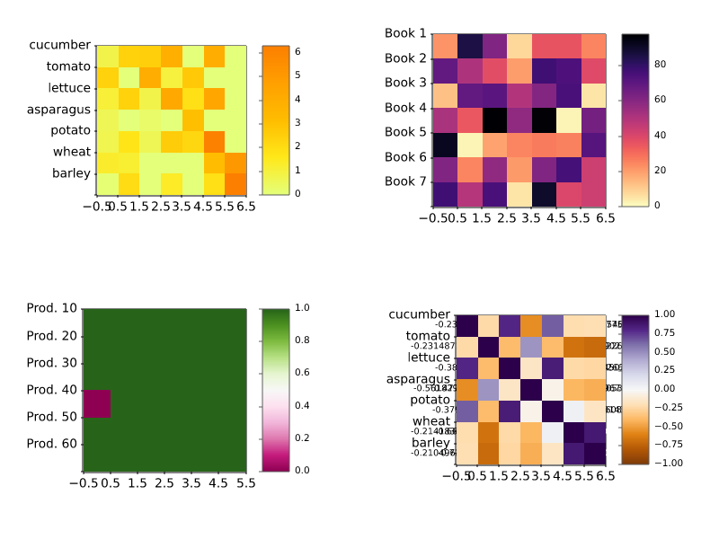
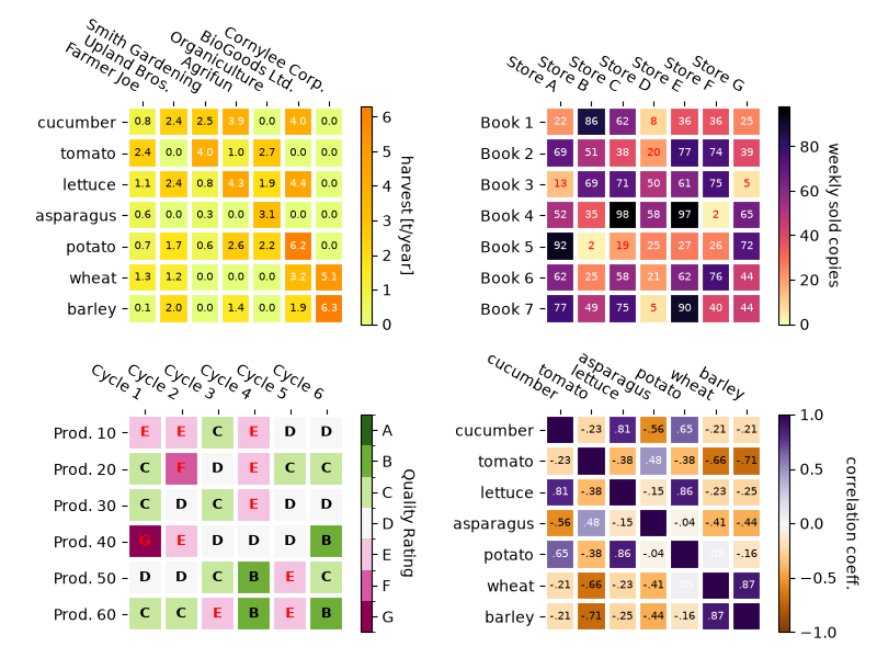
images_contours_and_fields/image_antialiasing
================
Source
"""
================
Image resampling
================

Images are represented by discrete pixels assigned color values, either on the
screen or in an image file.  When a user calls `~.Axes.imshow` with a data
array, it is rare that the size of the data array exactly matches the number of
pixels allotted to the image in the figure, so Matplotlib resamples or `scales
<https://en.wikipedia.org/wiki/Image_scaling>`_ the data or image to fit.  If
the data array is larger than the number of pixels allotted in the rendered figure,
then the image will be "down-sampled" and image information will be lost.
Conversely, if the data array is smaller than the number of output pixels then each
data point will get multiple pixels, and the image is "up-sampled".

In the following figure, the first data array has size (450, 450), but is
represented by far fewer pixels in the figure, and hence is down-sampled.  The
second data array has size (4, 4), and is represented by far more pixels, and
hence is up-sampled.
"""

import matplotlib.pyplot as plt
import numpy as np

fig, axs = plt.subplots(1, 2, figsize=(4, 2))

# First we generate a 450x450 pixel image with varying frequency content:
N = 450
x = np.arange(N) / N - 0.5
y = np.arange(N) / N - 0.5
aa = np.ones((N, N))
aa[::2, :] = -1

X, Y = np.meshgrid(x, y)
R = np.sqrt(X**2 + Y**2)
f0 = 5
k = 100
a = np.sin(np.pi * 2 * (f0 * R + k * R**2 / 2))
# make the left hand side of this
a[:int(N / 2), :][R[:int(N / 2), :] < 0.4] = -1
a[:int(N / 2), :][R[:int(N / 2), :] < 0.3] = 1
aa[:, int(N / 3):] = a[:, int(N / 3):]
alarge = aa

axs[0].imshow(alarge, cmap='RdBu_r')
axs[0].set_title('(450, 450) Down-sampled', fontsize='medium')

np.random.seed(19680801+9)
asmall = np.random.rand(4, 4)
axs[1].imshow(asmall, cmap='viridis')
axs[1].set_title('(4, 4) Up-sampled', fontsize='medium')

# %%
# Matplotlib's `~.Axes.imshow` method has two keyword arguments to allow the user
# to control how resampling is done.  The *interpolation* keyword argument allows
# a choice of the kernel that is used for resampling, allowing either `anti-alias
# <https://en.wikipedia.org/wiki/Anti-aliasing_filter>`_ filtering if
# down-sampling, or smoothing of pixels if up-sampling.  The
# *interpolation_stage* keyword argument, determines if this smoothing kernel is
# applied to the underlying data, or if the kernel is applied to the RGBA pixels.
#
# ``interpolation_stage='rgba'``: Data -> Normalize -> RGBA -> Interpolate/Resample
#
# ``interpolation_stage='data'``: Data -> Interpolate/Resample -> Normalize -> RGBA
#
# For both keyword arguments, Matplotlib has a default "auto", that is
# recommended for most situations, and is described below.  Note that this
# default behaves differently if the image is being down- or up-sampled, as
# described below.
#
# Down-sampling and modest up-sampling
# ====================================
#
# When down-sampling data, we usually want to remove aliasing by smoothing the
# image first and then sub-sampling it.  In Matplotlib, we can do that smoothing
# before mapping the data to colors, or we can do the smoothing on the RGB(A)
# image pixels.  The differences between these are shown below, and controlled
# with the *interpolation_stage* keyword argument.
#
# The following images are down-sampled from 450 data pixels to approximately
# 125 pixels or 250 pixels (depending on your display).
# The underlying image has alternating +1, -1 stripes on the left side, and
# a varying wavelength (`chirp <https://en.wikipedia.org/wiki/Chirp>`_) pattern
# in the rest of the image.  If we zoom, we can see this detail without any
# down-sampling:

fig, ax = plt.subplots(figsize=(4, 4), layout='compressed')
ax.imshow(alarge, interpolation='nearest', cmap='RdBu_r')
ax.set_xlim(100, 200)
ax.set_ylim(275, 175)
ax.set_title('Zoom')

# %%
# If we down-sample, the simplest algorithm is to decimate the data using
# `nearest-neighbor interpolation
# <https://en.wikipedia.org/wiki/Nearest-neighbor_interpolation>`_.  We can
# do this in either data space or RGBA space:

fig, axs = plt.subplots(1, 2, figsize=(5, 2.7), layout='compressed')
for ax, interp, space in zip(axs.flat, ['nearest', 'nearest'],
                                       ['data', 'rgba']):
    ax.imshow(alarge, interpolation=interp, interpolation_stage=space,
              cmap='RdBu_r')
    ax.set_title(f"interpolation='{interp}'\nstage='{space}'")

# %%
# Nearest interpolation is identical in data and RGBA space, and both exhibit
# `Moiré <https://en.wikipedia.org/wiki/Moiré_pattern>`_ patterns because the
# high-frequency data is being down-sampled and shows up as lower frequency
# patterns. We can reduce the Moiré patterns by applying an anti-aliasing filter
# to the image before rendering:

fig, axs = plt.subplots(1, 2, figsize=(5, 2.7), layout='compressed')
for ax, interp, space in zip(axs.flat, ['hanning', 'hanning'],
                                       ['data', 'rgba']):
    ax.imshow(alarge, interpolation=interp, interpolation_stage=space,
              cmap='RdBu_r')
    ax.set_title(f"interpolation='{interp}'\nstage='{space}'")
plt.show()

# %%
# The `Hanning <https://en.wikipedia.org/wiki/Hann_function>`_ filter smooths
# the underlying data so that each new pixel is a weighted average of the
# original underlying pixels.  This greatly reduces the Moiré patterns.
# However, when the *interpolation_stage* is set to 'data', it also introduces
# white regions to the image that are not in the original data, both in the
# alternating bands on the left hand side of the image, and in the boundary
# between the red and blue of the large circles in the middle of the image.
# The interpolation at the 'rgba' stage has a different artifact, with the alternating
# bands coming out a shade of purple; even though purple is not in the original
# colormap, it is what we perceive when a blue and red stripe are close to each
# other.
#
# The default for the *interpolation* keyword argument is 'auto' which
# will choose a Hanning filter if the image is being down-sampled or up-sampled
# by less than a factor of three.  The default *interpolation_stage* keyword
# argument is also 'auto', and for images that are down-sampled or
# up-sampled by less than a factor of three it defaults to 'rgba'
# interpolation.
#
# Anti-aliasing filtering is needed, even when up-sampling. The following image
# up-samples 450 data pixels to 530 rendered pixels. You may note a grid of
# line-like artifacts which stem from the extra pixels that had to be made up.
# Since interpolation is 'nearest' they are the same as a neighboring line of
# pixels and thus stretch the image locally so that it looks distorted.

fig, ax = plt.subplots(figsize=(6.8, 6.8))
ax.imshow(alarge, interpolation='nearest', cmap='grey')
ax.set_title("up-sampled by factor a 1.17, interpolation='nearest'")

# %%
# Better anti-aliasing algorithms can reduce this effect:
fig, ax = plt.subplots(figsize=(6.8, 6.8))
ax.imshow(alarge, interpolation='auto', cmap='grey')
ax.set_title("up-sampled by factor a 1.17, interpolation='auto'")

# %%
# Apart from the default 'hanning' anti-aliasing, `~.Axes.imshow` supports a
# number of different interpolation algorithms, which may work better or
# worse depending on the underlying data.
fig, axs = plt.subplots(1, 2, figsize=(7, 4), layout='constrained')
for ax, interp in zip(axs, ['hanning', 'lanczos']):
    ax.imshow(alarge, interpolation=interp, cmap='gray')
    ax.set_title(f"interpolation='{interp}'")

# %%
# A final example shows the desirability of performing the anti-aliasing at the
# RGBA stage when using non-trivial interpolation kernels.  In the following,
# the data in the outer circle is exactly 0.0, and data in the inner circle
# is exactly 2.0. If we perform the *interpolation_stage* in 'data' space and
# use an anti-aliasing filter (first panel), then floating point imprecision
# makes some of the data values just a bit less than zero or a bit more than
# 2.0, and they get assigned the under- or over- colors. This can be avoided if
# you do not use an anti-aliasing filter (*interpolation* set to
# 'nearest'), however, that makes the part of the data susceptible to Moiré
# patterns much worse (second panel).  Therefore, we recommend the default
# *interpolation* of 'hanning'/'auto', and *interpolation_stage* of
# 'rgba'/'auto' for most down-sampling situations (last panel).

a = alarge + 1
cmap = plt.get_cmap('RdBu_r')
cmap.set_under('yellow')
cmap.set_over('limegreen')

fig, axs = plt.subplots(1, 3, figsize=(7, 3), layout='constrained')
for ax, interp, space in zip(axs.flat,
                             ['hanning', 'nearest', 'hanning', ],
                             ['data', 'data', 'rgba']):
    im = ax.imshow(a, interpolation=interp, interpolation_stage=space,
                   cmap=cmap, vmin=0, vmax=2)
    title = f"interpolation='{interp}'\nstage='{space}'"
    if ax == axs[2]:
        title += '\nDefault'
    ax.set_title(title, fontsize='medium')
fig.colorbar(im, ax=axs, extend='both', shrink=0.8)

# %%
# Up-sampling
# ===========
#
# If we up-sample, then we can represent a data pixel by many image or screen pixels.
# In the following example, we greatly over-sample the small data matrix.

np.random.seed(19680801+9)
a = np.random.rand(4, 4)

fig, axs = plt.subplots(1, 2, figsize=(6.5, 4), layout='compressed')
axs[0].imshow(asmall, cmap='viridis')
axs[0].set_title("interpolation='auto'\nstage='auto'")
axs[1].imshow(asmall, cmap='viridis', interpolation="nearest",
              interpolation_stage="data")
axs[1].set_title("interpolation='nearest'\nstage='data'")
plt.show()

# %%
# The *interpolation* keyword argument can be used to smooth the pixels if desired.
# However, that almost always is better done in data space, rather than in RGBA space
# where the filters can cause colors that are not in the colormap to be the result of
# the interpolation.  In the following example, note that when the interpolation is
# 'rgba' there are red colors as interpolation artifacts.  Therefore, the default
# 'auto' choice for *interpolation_stage* is set to be the same as 'data'
# when up-sampling is greater than a factor of three:

fig, axs = plt.subplots(1, 2, figsize=(6.5, 4), layout='compressed')
im = axs[0].imshow(a, cmap='viridis', interpolation='sinc', interpolation_stage='data')
axs[0].set_title("interpolation='sinc'\nstage='data'\n(default for upsampling)")
axs[1].imshow(a, cmap='viridis', interpolation='sinc', interpolation_stage='rgba')
axs[1].set_title("interpolation='sinc'\nstage='rgba'")
fig.colorbar(im, ax=axs, shrink=0.7, extend='both')

# %%
# Avoiding resampling
# ===================
#
# It is possible to avoid resampling data when making an image.  One method is
# to simply save to a vector backend (pdf, eps, svg) and use
# ``interpolation='none'``.  Vector backends allow embedded images, however be
# aware that some vector image viewers may smooth image pixels.
#
# The second method is to exactly match the size of your axes to the size of
# your data. The following figure is exactly 2 inches by 2 inches, and
# if the dpi is 200, then the 400x400 data is not resampled at all. If you download
# this image and zoom in an image viewer you should see the individual stripes
# on the left hand side (note that if you have a non hiDPI or "retina" screen, the html
# may serve a 100x100 version of the image, which will be downsampled.)

fig = plt.figure(figsize=(2, 2))
ax = fig.add_axes((0, 0, 1, 1))
ax.imshow(aa[:400, :400], cmap='RdBu_r', interpolation='nearest')
plt.show()
# %%
#
# .. admonition:: References
#
#    The use of the following functions, methods, classes and modules is shown
#    in this example:
#
#    - `matplotlib.axes.Axes.imshow`
images_contours_and_fields/image_clip_path
============================
Source
"""
============================
Clipping images with patches
============================

Demo of image that's been clipped by a circular patch.
"""

from PIL import Image

import matplotlib.pyplot as plt

import matplotlib.cbook as cbook
import matplotlib.patches as patches

image = Image.open(cbook.get_sample_data("grace_hopper.jpg"))

fig, ax = plt.subplots()
im = ax.imshow(image)
patch = patches.Circle((260, 200), radius=200, transform=ax.transData)
im.set_clip_path(patch)

ax.axis('off')
plt.show()

# %%
#
# .. admonition:: References
#
#    The use of the following functions, methods, classes and modules is shown
#    in this example:
#
#    - `matplotlib.axes.Axes.imshow` / `matplotlib.pyplot.imshow`
#    - `matplotlib.artist.Artist.set_clip_path`

images_contours_and_fields/image_demo
========================
Source
"""
========================
Many ways to plot images
========================

The most common way to plot images in Matplotlib is with
`~.axes.Axes.imshow`. The following examples demonstrate much of the
functionality of imshow and the many images you can create.
"""

from PIL import Image

import matplotlib.pyplot as plt
import numpy as np

import matplotlib.cbook as cbook
from matplotlib.patches import PathPatch
from matplotlib.path import Path

# Fixing random state for reproducibility
np.random.seed(19680801)

# %%
# First we'll generate a simple bivariate normal distribution.

delta = 0.025
x = y = np.arange(-3.0, 3.0, delta)
X, Y = np.meshgrid(x, y)
Z1 = np.exp(-X**2 - Y**2)
Z2 = np.exp(-(X - 1)**2 - (Y - 1)**2)
Z = (Z1 - Z2) * 2

fig, ax = plt.subplots()
im = ax.imshow(Z, interpolation='bilinear', cmap="RdYlBu",
               origin='lower', extent=[-3, 3, -3, 3],
               vmax=abs(Z).max(), vmin=-abs(Z).max())

plt.show()


# %%
# It is also possible to show images of pictures.

# A sample image
image = Image.open(cbook.get_sample_data("grace_hopper.jpg"))

# And another image, using 256x256 16-bit integers.
w, h = 256, 256
with cbook.get_sample_data('s1045.ima.gz') as datafile:
    s = datafile.read()
A = np.frombuffer(s, np.uint16).astype(float).reshape((w, h))
extent = (0, 25, 0, 25)

fig, ax = plt.subplot_mosaic([
    ['hopper', 'mri']
], figsize=(7, 3.5))

ax['hopper'].imshow(image)
ax['hopper'].axis('off')  # clear x-axis and y-axis

im = ax['mri'].imshow(A, cmap="hot", origin='upper', extent=extent)

markers = [(15.9, 14.5), (16.8, 15)]
x, y = zip(*markers)
ax['mri'].plot(x, y, 'o')

ax['mri'].set_title('MRI')

plt.show()


# %%
# Interpolating images
# --------------------
#
# It is also possible to interpolate images before displaying them. Be careful,
# as this may manipulate the way your data looks, but it can be helpful for
# achieving the look you want. Below we'll display the same (small) array,
# interpolated with three different interpolation methods.
#
# The center of the pixel at A[i, j] is plotted at (i+0.5, i+0.5).  If you
# are using interpolation='nearest', the region bounded by (i, j) and
# (i+1, j+1) will have the same color.  If you are using interpolation,
# the pixel center will have the same color as it does with nearest, but
# other pixels will be interpolated between the neighboring pixels.
#
# To prevent edge effects when doing interpolation, Matplotlib pads the input
# array with identical pixels around the edge: if you have a 5x5 array with
# colors a-y as below::
#
#   a b c d e
#   f g h i j
#   k l m n o
#   p q r s t
#   u v w x y
#
# Matplotlib computes the interpolation and resizing on the padded array ::
#
#   a a b c d e e
#   a a b c d e e
#   f f g h i j j
#   k k l m n o o
#   p p q r s t t
#   o u v w x y y
#   o u v w x y y
#
# and then extracts the central region of the result.  (Extremely old versions
# of Matplotlib (<0.63) did not pad the array, but instead adjusted the view
# limits to hide the affected edge areas.)
#
# This approach allows plotting the full extent of an array without
# edge effects, and for example to layer multiple images of different
# sizes over one another with different interpolation methods -- see
# :doc:`/gallery/images_contours_and_fields/layer_images`.  It also implies
# a performance hit, as this new temporary, padded array must be created.
# Sophisticated interpolation also implies a performance hit; for maximal
# performance or very large images, interpolation='nearest' is suggested.

A = np.random.rand(5, 5)

fig, axs = plt.subplots(1, 3, figsize=(10, 3))
for ax, interp in zip(axs, ['nearest', 'bilinear', 'bicubic']):
    ax.imshow(A, interpolation=interp)
    ax.set_title(interp.capitalize())
    ax.grid(True)

plt.show()


# %%
# You can specify whether images should be plotted with the array origin
# x[0, 0] in the upper left or lower right by using the origin parameter.
# You can also control the default setting image.origin in your
# :ref:`matplotlibrc file <customizing-with-matplotlibrc-files>`. For more on
# this topic see the :ref:`complete guide on origin and extent
# <imshow_extent>`.

x = np.arange(120).reshape((10, 12))

interp = 'bilinear'
fig, axs = plt.subplots(nrows=2, sharex=True, figsize=(3, 5))
axs[0].set_title('blue should be up')
axs[0].imshow(x, origin='upper', interpolation=interp)

axs[1].set_title('blue should be down')
axs[1].imshow(x, origin='lower', interpolation=interp)
plt.show()


# %%
# Finally, we'll show an image using a clip path.

delta = 0.025
x = y = np.arange(-3.0, 3.0, delta)
X, Y = np.meshgrid(x, y)
Z1 = np.exp(-X**2 - Y**2)
Z2 = np.exp(-(X - 1)**2 - (Y - 1)**2)
Z = (Z1 - Z2) * 2

path = Path([[0, 1], [1, 0], [0, -1], [-1, 0], [0, 1]])
patch = PathPatch(path, facecolor='none')

fig, ax = plt.subplots()
ax.add_patch(patch)

im = ax.imshow(Z, interpolation='bilinear', cmap="gray",
               origin='lower', extent=[-3, 3, -3, 3],
               clip_path=patch, clip_on=True)
im.set_clip_path(patch)

plt.show()

# %%
#
# .. admonition:: References
#
#    The use of the following functions, methods, classes and modules is shown
#    in this example:
#
#    - `matplotlib.axes.Axes.imshow` / `matplotlib.pyplot.imshow`
#    - `matplotlib.artist.Artist.set_clip_path`
#    - `matplotlib.patches.PathPatch`
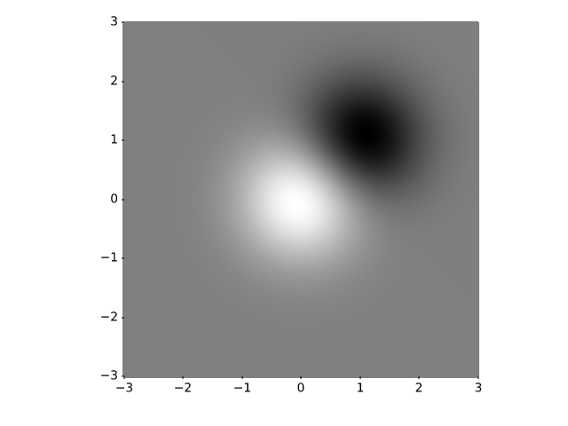
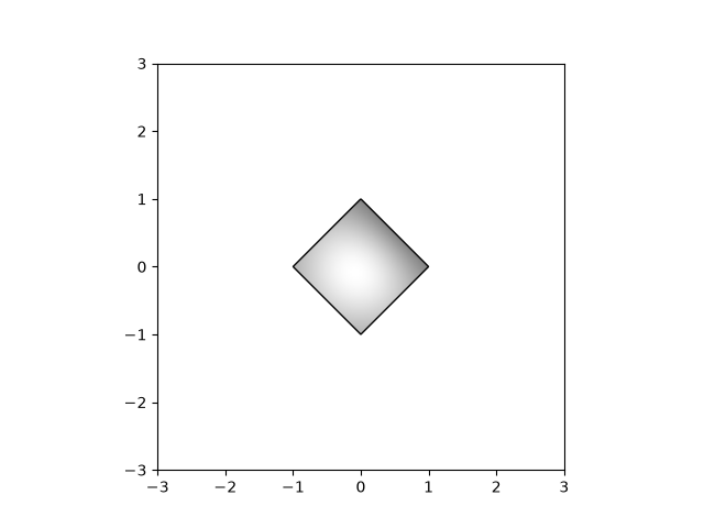
images_contours_and_fields/image_exact_placement
=========================================
Source
"""
=========================================
Placing images, preserving relative sizes
=========================================

By default Matplotlib resamples images created with `~.Axes.imshow` to
fit inside the parent `~.axes.Axes`.  This can mean that images that have very
different original sizes can end up appearing similar in size.

This example shows how to keep the images the same relative size, or
how to make the images keep exactly the same pixels as the original data.

Preserving relative sizes
=========================

By default the two images are made a similar size, despite one being 1.5 times the width
of the other:
"""

# sphinx_gallery_thumbnail_number = -1

import matplotlib.pyplot as plt
import numpy as np

import matplotlib.patches as mpatches

# make the data:
N = 450
x = np.arange(N) / N
y = np.arange(N) / N

X, Y = np.meshgrid(x, y)
R = np.sqrt(X**2 + Y**2)
f0 = 5
k = 100
a = np.sin(np.pi * 2 * (f0 * R + k * R**2 / 2))
A = a[:100, :300]
B = A[:40, :200]

# default layout: both axes have the same size
fig, axs = plt.subplots(1, 2, facecolor='aliceblue')

axs[0].imshow(A, vmin=-1, vmax=1)
axs[1].imshow(B, vmin=-1, vmax=1)


def annotate_rect(ax):
    # add a rectangle that is the size of the B matrix
    rect = mpatches.Rectangle((0, 0), 200, 40, linewidth=1,
                              edgecolor='r', facecolor='none')
    ax.add_patch(rect)
    return rect

annotate_rect(axs[0])

# %%
# Note that both images have an aspect ratio of 1 (i.e. pixels are square), but
# pixels sizes differ because the images are scaled to the same width.
#
# If the size of the images are amenable, we can preserve the relative sizes of two
# images by using either the *width_ratio* or *height_ratio* of the subplots.  Which
# one you use depends on the shape of the image and the size of the figure.
# We can control the relative sizes using the *width_ratios* argument *if* the images
# are wider than they are tall and shown side by side, as is the case here.
#
# While we are making changes, let us also make the aspect ratio of the figure closer
# to the aspect ratio of the axes using *figsize* so that the figure does not have so
# much white space. Note that you could alternatively trim extra blank space when
# saving a figure by passing ``bbox_inches="tight"`` to `~.Figure.savefig`.

fig, axs = plt.subplots(1, 2, width_ratios=[300/200, 1],
                        figsize=(6.4, 2), facecolor='aliceblue')

axs[0].imshow(A, vmin=-1, vmax=1)
annotate_rect(axs[0])

axs[1].imshow(B, vmin=-1, vmax=1)
# %%
# Given that the data subsample is in the upper left of the larger image,
# it might make sense if the top of the smaller Axes aligned with the top of the larger.
# This can be done manually by using `~.Axes.set_anchor`, and using "NW" (for
# northwest).

fig, axs = plt.subplots(1, 2, width_ratios=[300/200, 1],
                        figsize=(6.4, 2), facecolor='aliceblue')

axs[0].imshow(A, vmin=-1, vmax=1)
annotate_rect(axs[0])

axs[0].set_anchor('NW')
axs[1].imshow(B, vmin=-1, vmax=1)
axs[1].set_anchor('NW')

# %%
# Explicit placement
# ==================
# The above approach with adjusting ``figsize`` and ``width_ratios`` does
# not generalize well, because it needs manual parameter tuning, and
# possibly even code changes to using ``height_ratios`` instead of
# ``width_ratios`` depending on the aspects and layout of the images.
#
# We can alternative calculate positions explicitly and place Axes at absolute
# coordinates using `~.Figure.add_axes`. This takes the position in the form
# ``[left bottom width height]`` and is in
# :ref:`figure coordinates <transforms_tutorial>`. In the following, we
# determine figure size and Axes positions so that one image data point
# is rendered exactly to one figure pixel.

dpi = 100  # 100 pixels is one inch

# All variables from here are in pixels:
buffer = 0.35 * dpi  # pixels

# Get the position of A axes
left = buffer
bottom = buffer
ny, nx = np.shape(A)
posA = [left, bottom, nx, ny]
# we know this is tallest, so we can already get the fig height (in pixels)
fig_height = bottom + ny + buffer

# place the B axes to the right of the A axes
left = left + nx + buffer

ny, nx = np.shape(B)
# align the bottom so that the top lines up with the top of the A axes:
bottom = fig_height - buffer - ny
posB = [left, bottom, nx, ny]

# now we can get the fig width (in pixels)
fig_width = left + nx + buffer

# figsize must be in inches:
fig = plt.figure(figsize=(fig_width / dpi, fig_height / dpi), facecolor='aliceblue')

# the position posA must be normalized by the figure width and height:
ax = fig.add_axes((posA[0] / fig_width, posA[1] / fig_height,
                   posA[2] / fig_width, posA[3] / fig_height))
ax.imshow(A, vmin=-1, vmax=1)
annotate_rect(ax)

ax = fig.add_axes((posB[0] / fig_width, posB[1] / fig_height,
                   posB[2] / fig_width, posB[3] / fig_height))
ax.imshow(B, vmin=-1, vmax=1)
plt.show()
# %%
# Inspection of the image will show that it is exactly 3* 35 + 300 + 200 = 605
# pixels wide, and 2 * 35 + 100 = 170 pixels high (or twice that if the 2x
# version is used by the browser instead).  The images should be rendered with
# exactly 1 pixel per data point (or four, if 2x).
#
# .. admonition:: References
#
#    The use of the following functions, methods, classes and modules is shown
#    in this example:
#
#    - `matplotlib.axes.Axes.imshow`
#    - `matplotlib.figure.Figure.add_axes`
#
# .. tags::
#
#    component: figure
#    component: axes
#    styling: position
#    plot-type: image
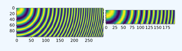
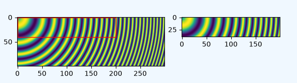
images_contours_and_fields/image_masked
========================
Source
"""
========================
Image with masked values
========================

imshow with masked array input and out-of-range colors.

The second subplot illustrates the use of BoundaryNorm to
get a filled contour effect.
"""

import matplotlib.pyplot as plt
import numpy as np

import matplotlib.colors as colors

# compute some interesting data
x0, x1 = -5, 5
y0, y1 = -3, 3
x = np.linspace(x0, x1, 500)
y = np.linspace(y0, y1, 500)
X, Y = np.meshgrid(x, y)
Z1 = np.exp(-X**2 - Y**2)
Z2 = np.exp(-(X - 1)**2 - (Y - 1)**2)
Z = (Z1 - Z2) * 2

# Set up a colormap:
palette = plt.colormaps["gray"].with_extremes(over='r', under='g', bad='b')
# Alternatively, we could use
# palette.set_bad(alpha = 0.0)
# to make the bad region transparent.  This is the default.
# If you comment out all the palette.set* lines, you will see
# all the defaults; under and over will be colored with the
# first and last colors in the palette, respectively.
Zm = np.ma.masked_where(Z > 1.2, Z)

# By setting vmin and vmax in the norm, we establish the
# range to which the regular palette color scale is applied.
# Anything above that range is colored based on palette.set_over, etc.

# set up the Axes objects
fig, (ax1, ax2) = plt.subplots(nrows=2, figsize=(6, 5.4))

# plot using 'continuous' colormap
im = ax1.imshow(Zm, interpolation='bilinear',
                cmap=palette,
                norm=colors.Normalize(vmin=-1.0, vmax=1.0),
                aspect='auto',
                origin='lower',
                extent=[x0, x1, y0, y1])
ax1.set_title('Green=low, Red=high, Blue=masked')
cbar = fig.colorbar(im, extend='both', shrink=0.9, ax=ax1)
cbar.set_label('uniform')
ax1.tick_params(axis='x', labelbottom=False)

# Plot using a small number of colors, with unevenly spaced boundaries.
im = ax2.imshow(Zm, interpolation='nearest',
                cmap=palette,
                norm=colors.BoundaryNorm([-1, -0.5, -0.2, 0, 0.2, 0.5, 1],
                                         ncolors=palette.N),
                aspect='auto',
                origin='lower',
                extent=[x0, x1, y0, y1])
ax2.set_title('With BoundaryNorm')
cbar = fig.colorbar(im, extend='both', spacing='proportional',
                    shrink=0.9, ax=ax2)
cbar.set_label('proportional')

fig.suptitle('imshow, with out-of-range and masked data')
plt.show()

# %%
#
# .. admonition:: References
#
#    The use of the following functions, methods, classes and modules is shown
#    in this example:
#
#    - `matplotlib.axes.Axes.imshow` / `matplotlib.pyplot.imshow`
#    - `matplotlib.figure.Figure.colorbar` / `matplotlib.pyplot.colorbar`
#    - `matplotlib.colors.BoundaryNorm`
#    - `matplotlib.colorbar.Colorbar.set_label`
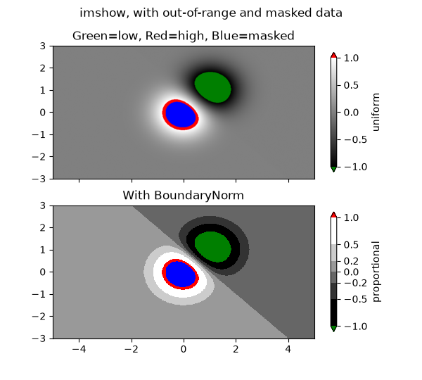
images_contours_and_fields/image_nonuniform
================
Source
"""
================
Image nonuniform
================

`.NonUniformImage` is a generalized image with pixels on a rectilinear grid,
i.e. it allows rows and columns with individual heights / widths.

There is no high-level plotting method on `~.axes.Axes` or `.pyplot` to
create a NonUniformImage. Instead, you have to instantiate the image
explicitly add it to the Axes using `.Axes.add_image`.
"""

import matplotlib.pyplot as plt
import numpy as np

from matplotlib.image import NonUniformImage

interp = 'nearest'

# Linear x array for cell centers:
x = np.linspace(-4, 4, 9)

# Highly nonlinear x array:
x2 = x**3

y = np.linspace(-4, 4, 9)

z = np.sqrt(x[np.newaxis, :]**2 + y[:, np.newaxis]**2)

fig, axs = plt.subplots(nrows=2, ncols=2, layout='constrained')
fig.suptitle('NonUniformImage class', fontsize='large')
ax = axs[0, 0]
im = NonUniformImage(ax, interpolation=interp, extent=(-4, 4, -4, 4),
                     cmap="Purples")
im.set_data(x, y, z)
ax.add_image(im)
ax.set_xlim(-4, 4)
ax.set_ylim(-4, 4)
ax.set_title(interp)

ax = axs[0, 1]
im = NonUniformImage(ax, interpolation=interp, extent=(-64, 64, -4, 4),
                     cmap="Purples")
im.set_data(x2, y, z)
ax.add_image(im)
ax.set_xlim(-64, 64)
ax.set_ylim(-4, 4)
ax.set_title(interp)

interp = 'bilinear'

ax = axs[1, 0]
im = NonUniformImage(ax, interpolation=interp, extent=(-4, 4, -4, 4),
                     cmap="Purples")
im.set_data(x, y, z)
ax.add_image(im)
ax.set_xlim(-4, 4)
ax.set_ylim(-4, 4)
ax.set_title(interp)

ax = axs[1, 1]
im = NonUniformImage(ax, interpolation=interp, extent=(-64, 64, -4, 4),
                     cmap="Purples")
im.set_data(x2, y, z)
ax.add_image(im)
ax.set_xlim(-64, 64)
ax.set_ylim(-4, 4)
ax.set_title(interp)

plt.show()
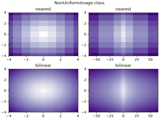
images_contours_and_fields/image_transparency_blend
==========================================
Source
"""
==========================================
Blend transparency with color in 2D images
==========================================

Blend transparency with color to highlight parts of data with imshow.

A common use for `matplotlib.pyplot.imshow` is to plot a 2D statistical
map. The function makes it easy to visualize a 2D matrix as an image and add
transparency to the output. For example, one can plot a statistic (such as a
t-statistic) and color the transparency of each pixel according to its p-value.
This example demonstrates how you can achieve this effect.

First we will generate some data, in this case, we'll create two 2D "blobs"
in a 2D grid. One blob will be positive, and the other negative.
"""

import matplotlib.pyplot as plt
# sphinx_gallery_thumbnail_number = 3
import numpy as np

from matplotlib.colors import Normalize


def normal_pdf(x, mean, var):
    return np.exp(-(x - mean)**2 / (2*var))


# Generate the space in which the blobs will live
xmin, xmax, ymin, ymax = (0, 100, 0, 100)
n_bins = 100
xx = np.linspace(xmin, xmax, n_bins)
yy = np.linspace(ymin, ymax, n_bins)

# Generate the blobs. The range of the values is roughly -.0002 to .0002
means_high = [20, 50]
means_low = [50, 60]
var = [150, 200]

gauss_x_high = normal_pdf(xx, means_high[0], var[0])
gauss_y_high = normal_pdf(yy, means_high[1], var[0])

gauss_x_low = normal_pdf(xx, means_low[0], var[1])
gauss_y_low = normal_pdf(yy, means_low[1], var[1])

weights = (np.outer(gauss_y_high, gauss_x_high)
           - np.outer(gauss_y_low, gauss_x_low))

# We'll also create a grey background into which the pixels will fade
greys = np.full((*weights.shape, 3), 70, dtype=np.uint8)

# First we'll plot these blobs using ``imshow`` without transparency.
vmax = np.abs(weights).max()
imshow_kwargs = {
    'vmax': vmax,
    'vmin': -vmax,
    'cmap': 'RdYlBu',
    'extent': (xmin, xmax, ymin, ymax),
}

fig, ax = plt.subplots()
ax.imshow(greys)
ax.imshow(weights, **imshow_kwargs)
ax.set_axis_off()

# %%
# Blending in transparency
# ========================
#
# The simplest way to include transparency when plotting data with
# `matplotlib.pyplot.imshow` is to pass an array matching the shape of
# the data to the ``alpha`` argument. For example, we'll create a gradient
# moving from left to right below.

# Create an alpha channel of linearly increasing values moving to the right.
alphas = np.ones(weights.shape)
alphas[:, 30:] = np.linspace(1, 0, 70)

# Create the figure and image
# Note that the absolute values may be slightly different
fig, ax = plt.subplots()
ax.imshow(greys)
ax.imshow(weights, alpha=alphas, **imshow_kwargs)
ax.set_axis_off()

# %%
# Using transparency to highlight values with high amplitude
# ==========================================================
#
# Finally, we'll recreate the same plot, but this time we'll use transparency
# to highlight the extreme values in the data. This is often used to highlight
# data points with smaller p-values. We'll also add in contour lines to
# highlight the image values.

# Create an alpha channel based on weight values
# Any value whose absolute value is > .0001 will have zero transparency
alphas = Normalize(0, .3, clip=True)(np.abs(weights))
alphas = np.clip(alphas, .4, 1)  # alpha value clipped at the bottom at .4

# Create the figure and image
# Note that the absolute values may be slightly different
fig, ax = plt.subplots()
ax.imshow(greys)
ax.imshow(weights, alpha=alphas, **imshow_kwargs)

# Add contour lines to further highlight different levels.
ax.contour(weights[::-1], levels=[-.1, .1], colors='k', linestyles='-')
ax.set_axis_off()
plt.show()

ax.contour(weights[::-1], levels=[-.0001, .0001], colors='k', linestyles='-')
ax.set_axis_off()
plt.show()

# %%
#
# .. admonition:: References
#
#    The use of the following functions, methods, classes and modules is shown
#    in this example:
#
#    - `matplotlib.axes.Axes.imshow` / `matplotlib.pyplot.imshow`
#    - `matplotlib.axes.Axes.contour` / `matplotlib.pyplot.contour`
#    - `matplotlib.colors.Normalize`
#    - `matplotlib.axes.Axes.set_axis_off`
images_contours_and_fields/image_zcoord
==================================
Source
"""
==================================
Modifying the coordinate formatter
==================================

Modify the coordinate formatter to report the image "z" value of the nearest
pixel given x and y.  This functionality is built in by default; this example
just showcases how to customize the `~.axes.Axes.format_coord` function.
"""

import matplotlib.pyplot as plt
import numpy as np

# Fixing random state for reproducibility
np.random.seed(19680801)


X = 10*np.random.rand(5, 3)

fig, ax = plt.subplots()
ax.imshow(X)


def format_coord(x, y):
    col = round(x)
    row = round(y)
    nrows, ncols = X.shape
    if 0 <= col < ncols and 0 <= row < nrows:
        z = X[row, col]
        return f'x={x:1.4f}, y={y:1.4f}, z={z:1.4f}'
    else:
        return f'x={x:1.4f}, y={y:1.4f}'


ax.format_coord = format_coord
plt.show()

# %%
#
# .. admonition:: References
#
#    The use of the following functions, methods, classes and modules is shown
#    in this example:
#
#    - `matplotlib.axes.Axes.format_coord`
#    - `matplotlib.axes.Axes.imshow`
images_contours_and_fields/interpolation_methods
=========================
Source
"""
=========================
Interpolations for imshow
=========================

This example displays the difference between interpolation methods for
`~.axes.Axes.imshow`.

If *interpolation* is None, it defaults to the :rc:`image.interpolation`.
If the interpolation is ``'none'``, then no interpolation is performed for the
Agg, ps and pdf backends. Other backends will default to ``'auto'``.

For the Agg, ps and pdf backends, ``interpolation='none'`` works well when a
big image is scaled down, while ``interpolation='nearest'`` works well when
a small image is scaled up.

See :doc:`/gallery/images_contours_and_fields/image_antialiasing` for a
discussion on the default ``interpolation='auto'`` option.
"""

import matplotlib.pyplot as plt
import numpy as np

methods = [None, 'none', 'nearest', 'bilinear', 'bicubic', 'spline16',
           'spline36', 'hanning', 'hamming', 'hermite', 'kaiser', 'quadric',
           'catrom', 'gaussian', 'bessel', 'mitchell', 'sinc', 'lanczos']

# Fixing random state for reproducibility
np.random.seed(19680801)

grid = np.random.rand(4, 4)

fig, axs = plt.subplots(nrows=3, ncols=6, figsize=(9, 6),
                        subplot_kw={'xticks': [], 'yticks': []})

for ax, interp_method in zip(axs.flat, methods):
    ax.imshow(grid, interpolation=interp_method, cmap='viridis')
    ax.set_title(str(interp_method))

plt.tight_layout()
plt.show()

# %%
#
# .. admonition:: References
#
#    The use of the following functions, methods, classes and modules is shown
#    in this example:
#
#    - `matplotlib.axes.Axes.imshow` / `matplotlib.pyplot.imshow`
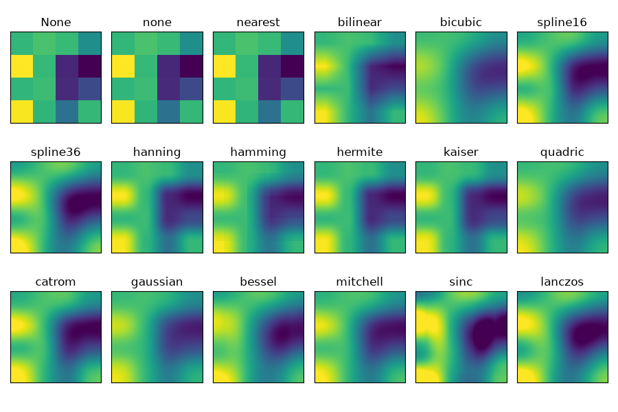
images_contours_and_fields/irregulardatagrid
=======================================
Source
"""
=======================================
Contour plot of irregularly spaced data
=======================================

Comparison of a contour plot of irregularly spaced data interpolated
on a regular grid versus a tricontour plot for an unstructured triangular grid.

Since `~.axes.Axes.contour` and `~.axes.Axes.contourf` expect the data to live
on a regular grid, plotting a contour plot of irregularly spaced data requires
different methods. The two options are:

* Interpolate the data to a regular grid first. This can be done with on-board
  means, e.g. via `~.tri.LinearTriInterpolator` or using external functionality
  e.g. via `scipy.interpolate.griddata`. Then plot the interpolated data with
  the usual `~.axes.Axes.contour`.
* Directly use `~.axes.Axes.tricontour` or `~.axes.Axes.tricontourf` which will
  perform a triangulation internally.

This example shows both methods in action.
"""

import matplotlib.pyplot as plt
import numpy as np

import matplotlib.tri as tri

np.random.seed(19680801)
npts = 200
ngridx = 100
ngridy = 200
x = np.random.uniform(-2, 2, npts)
y = np.random.uniform(-2, 2, npts)
z = x * np.exp(-x**2 - y**2)

fig, (ax1, ax2) = plt.subplots(nrows=2)

# -----------------------
# Interpolation on a grid
# -----------------------
# A contour plot of irregularly spaced data coordinates
# via interpolation on a grid.

# Create grid values first.
xi = np.linspace(-2.1, 2.1, ngridx)
yi = np.linspace(-2.1, 2.1, ngridy)

# Linearly interpolate the data (x, y) on a grid defined by (xi, yi).
triang = tri.Triangulation(x, y)
interpolator = tri.LinearTriInterpolator(triang, z)
Xi, Yi = np.meshgrid(xi, yi)
zi = interpolator(Xi, Yi)

# Note that scipy.interpolate provides means to interpolate data on a grid
# as well. The following would be an alternative to the four lines above:
# from scipy.interpolate import griddata
# zi = griddata((x, y), z, (xi[None, :], yi[:, None]), method='linear')

ax1.contour(xi, yi, zi, levels=14, linewidths=0.5, colors='k')
cntr1 = ax1.contourf(xi, yi, zi, levels=14, cmap="RdBu_r")

fig.colorbar(cntr1, ax=ax1)
ax1.plot(x, y, 'ko', ms=3)
ax1.set(xlim=(-2, 2), ylim=(-2, 2))
ax1.set_title('grid and contour (%d points, %d grid points)' %
              (npts, ngridx * ngridy))

# ----------
# Tricontour
# ----------
# Directly supply the unordered, irregularly spaced coordinates
# to tricontour.

ax2.tricontour(x, y, z, levels=14, linewidths=0.5, colors='k')
cntr2 = ax2.tricontourf(x, y, z, levels=14, cmap="RdBu_r")

fig.colorbar(cntr2, ax=ax2)
ax2.plot(x, y, 'ko', ms=3)
ax2.set(xlim=(-2, 2), ylim=(-2, 2))
ax2.set_title('tricontour (%d points)' % npts)

plt.subplots_adjust(hspace=0.5)
plt.show()

# %%
#
# .. admonition:: References
#
#    The use of the following functions, methods, classes and modules is shown
#    in this example:
#
#    - `matplotlib.axes.Axes.contour` / `matplotlib.pyplot.contour`
#    - `matplotlib.axes.Axes.contourf` / `matplotlib.pyplot.contourf`
#    - `matplotlib.axes.Axes.tricontour` / `matplotlib.pyplot.tricontour`
#    - `matplotlib.axes.Axes.tricontourf` / `matplotlib.pyplot.tricontourf`
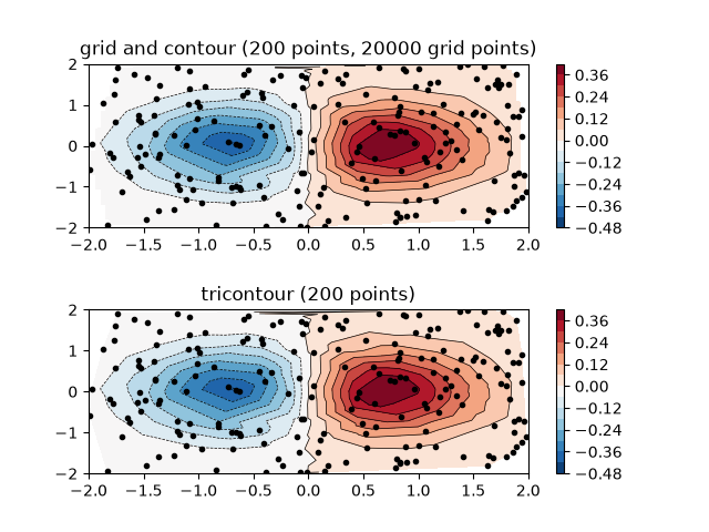
images_contours_and_fields/layer_images
================================
Source
"""
================================
Layer images with alpha blending
================================

Layer images above one another using alpha blending
"""
import matplotlib.pyplot as plt
import numpy as np


def func3(x, y):
    return (1 - x / 2 + x**5 + y**3) * np.exp(-(x**2 + y**2))


# make these smaller to increase the resolution
dx, dy = 0.05, 0.05

x = np.arange(-3.0, 3.0, dx)
y = np.arange(-3.0, 3.0, dy)
X, Y = np.meshgrid(x, y)

# when layering multiple images, the images need to have the same
# extent.  This does not mean they need to have the same shape, but
# they both need to render to the same coordinate system determined by
# xmin, xmax, ymin, ymax.  Note if you use different interpolations
# for the images their apparent extent could be different due to
# interpolation edge effects

extent = np.min(x), np.max(x), np.min(y), np.max(y)
fig = plt.figure(frameon=False)

Z1 = np.add.outer(range(8), range(8)) % 2  # chessboard
im1 = plt.imshow(Z1, cmap="gray", interpolation='nearest',
                 extent=extent)

Z2 = func3(X, Y)

im2 = plt.imshow(Z2, cmap="viridis", alpha=.9, interpolation='bilinear',
                 extent=extent)

plt.show()

# %%
#
# .. admonition:: References
#
#    The use of the following functions, methods, classes and modules is shown
#    in this example:
#
#    - `matplotlib.axes.Axes.imshow` / `matplotlib.pyplot.imshow`
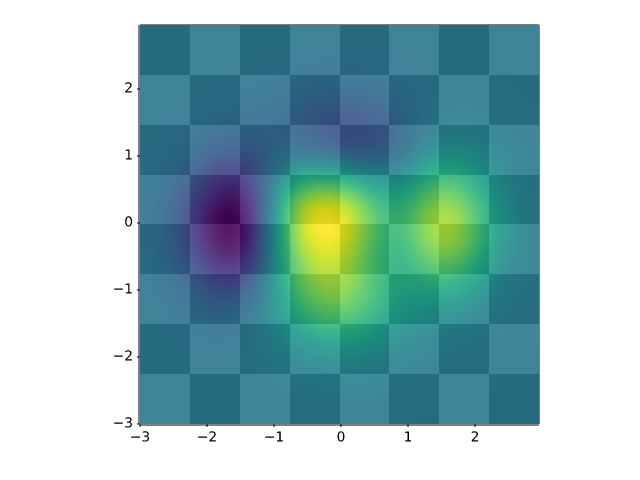
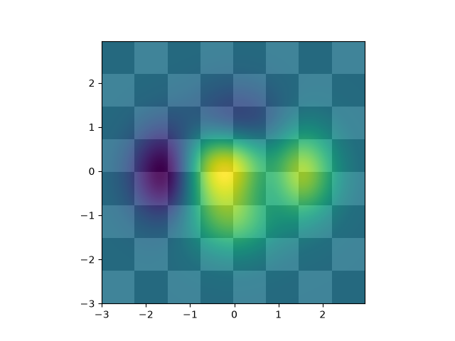
images_contours_and_fields/matshow
===============================
Source
"""
===============================
Visualize matrices with matshow
===============================

`~.axes.Axes.matshow` visualizes a 2D matrix or array as color-coded image.
"""
import matplotlib.pyplot as plt
import numpy as np

# a 2D array with linearly increasing values on the diagonal
a = np.diag(range(15))

plt.matshow(a)

plt.show()

# %%
#
# .. admonition:: References
#
#    The use of the following functions, methods, classes and modules is shown
#    in this example:
#
#    - `matplotlib.axes.Axes.imshow` / `matplotlib.pyplot.imshow`
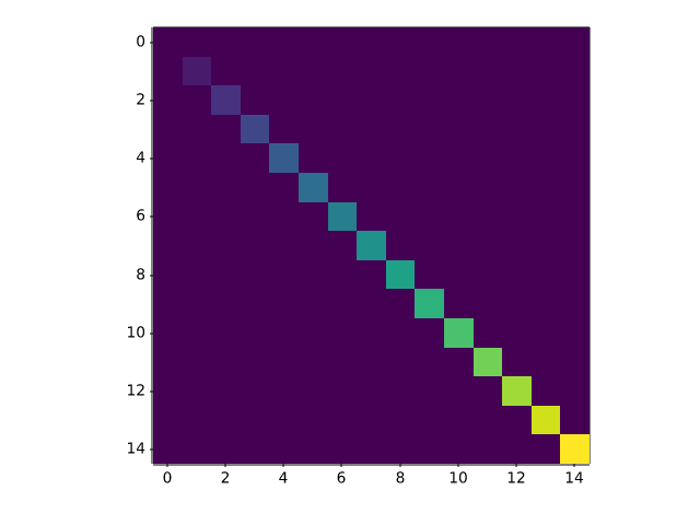
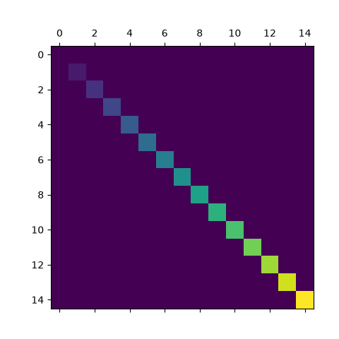
images_contours_and_fields/multi_image
=================================
Source
"""
=================================
Multiple images with one colorbar
=================================

Use a single colorbar for multiple images.

Currently, a colorbar can only be connected to one image. The connection
guarantees that the data coloring is consistent with the colormap scale
(i.e. the color of value *x* in the colormap is used for coloring a data
value *x* in the image).

If we want one colorbar to be representative for multiple images, we have
to explicitly ensure consistent data coloring by using the same
data-to-color pipeline for all the images. We ensure this by explicitly
creating a `matplotlib.colorizer.Colorizer` object that we pass to all
the image plotting methods.
"""

import matplotlib.pyplot as plt
import numpy as np

import matplotlib.colorizer as mcolorizer
import matplotlib.colors as mcolors

np.random.seed(19680801)

datasets = [
    (i+1)/10 * np.random.rand(10, 20)
    for i in range(4)
]

fig, axs = plt.subplots(2, 2)
fig.suptitle('Multiple images')

# create a colorizer with a predefined norm to be shared across all images
norm = mcolors.Normalize(vmin=np.min(datasets), vmax=np.max(datasets))
colorizer = mcolorizer.Colorizer(norm=norm)

images = []
for ax, data in zip(axs.flat, datasets):
    images.append(ax.imshow(data, colorizer=colorizer))

fig.colorbar(images[0], ax=axs, orientation='horizontal', fraction=.1)

plt.show()

# %%
# The colors are now kept consistent across all images when changing the
# scaling, e.g. through zooming in the colorbar or via the "edit axis,
# curves and images parameters" GUI of the Qt backend. Additionally,
# if the colormap of the colorizer is changed, (e.g. through the "edit
# axis, curves and images parameters" GUI of the Qt backend) this change
# propagates to the other plots and the colorbar.
#
# .. admonition:: References
#
#    The use of the following functions, methods, classes and modules is shown
#    in this example:
#
#    - `matplotlib.axes.Axes.imshow` / `matplotlib.pyplot.imshow`
#    - `matplotlib.figure.Figure.colorbar` / `matplotlib.pyplot.colorbar`
#    - `matplotlib.colorizer.Colorizer`
#    - `matplotlib.colors.Normalize`
images_contours_and_fields/pcolor_demo
=============
Source
"""
=============
pcolor images
=============

`~.Axes.pcolor` generates 2D image-style plots, as illustrated below.
"""

import matplotlib.pyplot as plt
import numpy as np

from matplotlib.colors import LogNorm

# Fixing random state for reproducibility
np.random.seed(19680801)

# %%
# A simple pcolor demo
# --------------------

Z = np.random.rand(6, 10)

fig, (ax0, ax1) = plt.subplots(2, 1)

c = ax0.pcolor(Z)
ax0.set_title('default: no edges')

c = ax1.pcolor(Z, edgecolors='k', linewidths=4)
ax1.set_title('thick edges')

fig.tight_layout()
plt.show()

# %%
# Comparing pcolor with similar functions
# ---------------------------------------
#
# Demonstrates similarities between `~.axes.Axes.pcolor`,
# `~.axes.Axes.pcolormesh`, `~.axes.Axes.imshow` and
# `~.axes.Axes.pcolorfast` for drawing quadrilateral grids.
# Note that we call ``imshow`` with ``aspect="auto"`` so that it doesn't force
# the data pixels to be square (the default is ``aspect="equal"``).

# make these smaller to increase the resolution
dx, dy = 0.15, 0.05

# generate 2 2d grids for the x & y bounds
y, x = np.mgrid[-3:3+dy:dy, -3:3+dx:dx]
z = (1 - x/2 + x**5 + y**3) * np.exp(-x**2 - y**2)
# x and y are bounds, so z should be the value *inside* those bounds.
# Therefore, remove the last value from the z array.
z = z[:-1, :-1]
z_min, z_max = -abs(z).max(), abs(z).max()

fig, axs = plt.subplots(2, 2)

ax = axs[0, 0]
c = ax.pcolor(x, y, z, cmap='RdBu', vmin=z_min, vmax=z_max)
ax.set_title('pcolor')
fig.colorbar(c, ax=ax)

ax = axs[0, 1]
c = ax.pcolormesh(x, y, z, cmap='RdBu', vmin=z_min, vmax=z_max)
ax.set_title('pcolormesh')
fig.colorbar(c, ax=ax)

ax = axs[1, 0]
c = ax.imshow(z, cmap='RdBu', vmin=z_min, vmax=z_max,
              extent=[x.min(), x.max(), y.min(), y.max()],
              interpolation='nearest', origin='lower', aspect='auto')
ax.set_title('image (nearest, aspect="auto")')
fig.colorbar(c, ax=ax)

ax = axs[1, 1]
c = ax.pcolorfast(x, y, z, cmap='RdBu', vmin=z_min, vmax=z_max)
ax.set_title('pcolorfast')
fig.colorbar(c, ax=ax)

fig.tight_layout()
plt.show()


# %%
# Pcolor with a log scale
# -----------------------
#
# The following shows pcolor plots with a log scale.

N = 100
X, Y = np.meshgrid(np.linspace(-3, 3, N), np.linspace(-2, 2, N))

# A low hump with a spike coming out.
# Needs to have z/colour axis on a log scale, so we see both hump and spike.
# A linear scale only shows the spike.
Z1 = np.exp(-X**2 - Y**2)
Z2 = np.exp(-(X * 10)**2 - (Y * 10)**2)
Z = Z1 + 50 * Z2

fig, (ax0, ax1) = plt.subplots(2, 1)

c = ax0.pcolor(X, Y, Z, shading='auto',
               norm=LogNorm(vmin=Z.min(), vmax=Z.max()), cmap='PuBu_r')
fig.colorbar(c, ax=ax0)

c = ax1.pcolor(X, Y, Z, cmap='PuBu_r', shading='auto')
fig.colorbar(c, ax=ax1)

plt.show()

# %%
#
# .. admonition:: References
#
#    The use of the following functions, methods, classes and modules is shown
#    in this example:
#
#    - `matplotlib.axes.Axes.pcolor` / `matplotlib.pyplot.pcolor`
#    - `matplotlib.axes.Axes.pcolormesh` / `matplotlib.pyplot.pcolormesh`
#    - `matplotlib.axes.Axes.pcolorfast`
#    - `matplotlib.axes.Axes.imshow` / `matplotlib.pyplot.imshow`
#    - `matplotlib.figure.Figure.colorbar` / `matplotlib.pyplot.colorbar`
#    - `matplotlib.colors.LogNorm`
images_contours_and_fields/pcolormesh_grids
============================
Source
"""
============================
pcolormesh grids and shading
============================

`.axes.Axes.pcolormesh` and `~.axes.Axes.pcolor` have a few options for
how grids are laid out and the shading between the grid points.

Generally, if *Z* has shape *(M, N)* then the grid *X* and *Y* can be
specified with either shape *(M+1, N+1)* or *(M, N)*, depending on the
argument for the ``shading`` keyword argument.  Note that below we specify
vectors *x* as either length N or N+1 and *y* as length M or M+1, and
`~.axes.Axes.pcolormesh` internally makes the mesh matrices *X* and *Y* from
the input vectors.

"""

import matplotlib.pyplot as plt
import numpy as np

# %%
# Flat Shading
# ------------
#
# The grid specification with the least assumptions is ``shading='flat'``
# and if the grid is one larger than the data in each dimension, i.e. has shape
# *(M+1, N+1)*.  In that case *X* and *Y* specify the corners of quadrilaterals
# that are colored with the values in *Z*. Here we specify the edges of the
# *(3, 5)* quadrilaterals with *X* and *Y* that are *(4, 6)*.

nrows = 3
ncols = 5
Z = np.arange(nrows * ncols).reshape(nrows, ncols)
x = np.arange(ncols + 1)
y = np.arange(nrows + 1)

fig, ax = plt.subplots()
ax.pcolormesh(x, y, Z, shading='flat', vmin=Z.min(), vmax=Z.max())


def _annotate(ax, x, y, title):
    # this all gets repeated below:
    X, Y = np.meshgrid(x, y)
    ax.plot(X.flat, Y.flat, 'o', color='m')
    ax.set_xlim(-0.7, 5.2)
    ax.set_ylim(-0.7, 3.2)
    ax.set_title(title)

_annotate(ax, x, y, "shading='flat'")


# %%
# Flat Shading, same shape grid
# -----------------------------
#
# Often, however, data is provided where *X* and *Y* match the shape of *Z*.
# While this makes sense for other ``shading`` types, it is not permitted
# when ``shading='flat'``. Historically, Matplotlib silently dropped the last
# row and column of *Z* in this case, to match Matlab's behavior. If this
# behavior is still desired, simply drop the last row and column manually:

x = np.arange(ncols)  # note *not* ncols + 1 as before
y = np.arange(nrows)
fig, ax = plt.subplots()
ax.pcolormesh(x, y, Z[:-1, :-1], shading='flat', vmin=Z.min(), vmax=Z.max())
_annotate(ax, x, y, "shading='flat': X, Y, C same shape")

# %%
# Nearest Shading, same shape grid
# --------------------------------
#
# Usually, dropping a row and column of data is not what the user means when
# they make *X*, *Y* and *Z* all the same shape.  For this case, Matplotlib
# allows ``shading='nearest'`` and centers the colored quadrilaterals on the
# grid points.
#
# If a grid that is not the correct shape is passed with ``shading='nearest'``
# an error is raised.

fig, ax = plt.subplots()
ax.pcolormesh(x, y, Z, shading='nearest', vmin=Z.min(), vmax=Z.max())
_annotate(ax, x, y, "shading='nearest'")

# %%
# Auto Shading
# ------------
#
# It's possible that the user would like the code to automatically choose which
# to use, in this case ``shading='auto'`` will decide whether to use 'flat' or
# 'nearest' shading based on the shapes of *X*, *Y* and *Z*.

fig, axs = plt.subplots(2, 1, layout='constrained')
ax = axs[0]
x = np.arange(ncols)
y = np.arange(nrows)
ax.pcolormesh(x, y, Z, shading='auto', vmin=Z.min(), vmax=Z.max())
_annotate(ax, x, y, "shading='auto'; X, Y, Z: same shape (nearest)")

ax = axs[1]
x = np.arange(ncols + 1)
y = np.arange(nrows + 1)
ax.pcolormesh(x, y, Z, shading='auto', vmin=Z.min(), vmax=Z.max())
_annotate(ax, x, y, "shading='auto'; X, Y one larger than Z (flat)")

# %%
# Gouraud Shading
# ---------------
#
# `Gouraud shading <https://en.wikipedia.org/wiki/Gouraud_shading>`_ can also
# be specified, where the color in the quadrilaterals is linearly interpolated
# between the grid points.  The shapes of *X*, *Y*, *Z* must be the same.

fig, ax = plt.subplots(layout='constrained')
x = np.arange(ncols)
y = np.arange(nrows)
ax.pcolormesh(x, y, Z, shading='gouraud', vmin=Z.min(), vmax=Z.max())
_annotate(ax, x, y, "shading='gouraud'; X, Y same shape as Z")

plt.show()
# %%
#
# .. admonition:: References
#
#    The use of the following functions, methods, classes and modules is shown
#    in this example:
#
#    - `matplotlib.axes.Axes.pcolormesh` / `matplotlib.pyplot.pcolormesh`
images_contours_and_fields/pcolormesh_levels
==========
Source
"""
==========
pcolormesh
==========

`.axes.Axes.pcolormesh` allows you to generate 2D image-style plots.
Note that it is faster than the similar `~.axes.Axes.pcolor`.

"""

import matplotlib.pyplot as plt
import numpy as np

from matplotlib.colors import BoundaryNorm
from matplotlib.ticker import MaxNLocator

# %%
# Basic pcolormesh
# ----------------
#
# We usually specify a pcolormesh by defining the edge of quadrilaterals and
# the value of the quadrilateral.  Note that here *x* and *y* each have one
# extra element than Z in the respective dimension.

np.random.seed(19680801)
Z = np.random.rand(6, 10)
x = np.arange(-0.5, 10, 1)  # len = 11
y = np.arange(4.5, 11, 1)  # len = 7

fig, ax = plt.subplots()
ax.pcolormesh(x, y, Z)

# %%
# Non-rectilinear pcolormesh
# --------------------------
#
# Note that we can also specify matrices for *X* and *Y* and have
# non-rectilinear quadrilaterals.

x = np.arange(-0.5, 10, 1)  # len = 11
y = np.arange(4.5, 11, 1)  # len = 7
X, Y = np.meshgrid(x, y)
X = X + 0.2 * Y  # tilt the coordinates.
Y = Y + 0.3 * X

fig, ax = plt.subplots()
ax.pcolormesh(X, Y, Z)

# %%
# Centered Coordinates
# ---------------------
#
# Often a user wants to pass *X* and *Y* with the same sizes as *Z* to
# `.axes.Axes.pcolormesh`. This is also allowed if ``shading='auto'`` is
# passed (default set by :rc:`pcolor.shading`). Pre Matplotlib 3.3,
# ``shading='flat'`` would drop the last column and row of *Z*, but now gives
# an error. If this is really what you want, then simply drop the last row and
# column of Z manually:

x = np.arange(10)  # len = 10
y = np.arange(6)  # len = 6
X, Y = np.meshgrid(x, y)

fig, axs = plt.subplots(2, 1, sharex=True, sharey=True)
axs[0].pcolormesh(X, Y, Z, vmin=np.min(Z), vmax=np.max(Z), shading='auto')
axs[0].set_title("shading='auto' = 'nearest'")
axs[1].pcolormesh(X, Y, Z[:-1, :-1], vmin=np.min(Z), vmax=np.max(Z),
                  shading='flat')
axs[1].set_title("shading='flat'")

# %%
# Making levels using Norms
# -------------------------
#
# Shows how to combine Normalization and Colormap instances to draw
# "levels" in `.axes.Axes.pcolor`, `.axes.Axes.pcolormesh`
# and `.axes.Axes.imshow` type plots in a similar
# way to the levels keyword argument to contour/contourf.

# make these smaller to increase the resolution
dx, dy = 0.05, 0.05

# generate 2 2d grids for the x & y bounds
y, x = np.mgrid[slice(1, 5 + dy, dy),
                slice(1, 5 + dx, dx)]

z = np.sin(x)**10 + np.cos(10 + y*x) * np.cos(x)

# x and y are bounds, so z should be the value *inside* those bounds.
# Therefore, remove the last value from the z array.
z = z[:-1, :-1]
levels = MaxNLocator(nbins=15).tick_values(z.min(), z.max())


# pick the desired colormap, sensible levels, and define a normalization
# instance which takes data values and translates those into levels.
cmap = plt.colormaps['PiYG']
norm = BoundaryNorm(levels, ncolors=cmap.N, clip=True)

fig, (ax0, ax1) = plt.subplots(nrows=2)

im = ax0.pcolormesh(x, y, z, cmap=cmap, norm=norm)
fig.colorbar(im, ax=ax0)
ax0.set_title('pcolormesh with levels')


# contours are *point* based plots, so convert our bound into point
# centers
cf = ax1.contourf(x[:-1, :-1] + dx/2.,
                  y[:-1, :-1] + dy/2., z, levels=levels,
                  cmap=cmap)
fig.colorbar(cf, ax=ax1)
ax1.set_title('contourf with levels')

# adjust spacing between subplots so `ax1` title and `ax0` tick labels
# don't overlap
fig.tight_layout()

plt.show()

# %%
#
# .. admonition:: References
#
#    The use of the following functions, methods, classes and modules is shown
#    in this example:
#
#    - `matplotlib.axes.Axes.pcolormesh` / `matplotlib.pyplot.pcolormesh`
#    - `matplotlib.axes.Axes.contourf` / `matplotlib.pyplot.contourf`
#    - `matplotlib.figure.Figure.colorbar` / `matplotlib.pyplot.colorbar`
#    - `matplotlib.colors.BoundaryNorm`
#    - `matplotlib.ticker.MaxNLocator`
images_contours_and_fields/plot_streamplot
==========
Source
"""
==========
Streamplot
==========

A stream plot, or streamline plot, is used to display 2D vector fields. This
example shows a few features of the `~.axes.Axes.streamplot` function:

* Varying the color along a streamline.
* Varying the density of streamlines.
* Varying the line width along a streamline.
* Controlling the starting points of streamlines.
* Streamlines skipping masked regions and NaN values.
* Unbroken streamlines even when exceeding the limit of lines within a single
  grid cell.
"""
import time

import matplotlib.pyplot as plt
import numpy as np

w = 3
Y, X = np.mgrid[-w:w:100j, -w:w:100j]
U = -1 - X**2 + Y
V = 1 + X - Y**2
speed = np.sqrt(U**2 + V**2)

fig, axs = plt.subplots(4, 2, figsize=(7, 12), height_ratios=[1, 1, 1, 2])
axs = axs.flat

#  Varying density along a streamline
axs[0].streamplot(X, Y, U, V, density=[0.5, 1])
axs[0].set_title('Varying Density')

# Varying color along a streamline
strm = axs[1].streamplot(X, Y, U, V, color=U, linewidth=2, cmap='autumn')
fig.colorbar(strm.lines)
axs[1].set_title('Varying Color')

#  Varying line width along a streamline
lw = 5*speed / speed.max()
axs[2].streamplot(X, Y, U, V, density=0.6, color='k', linewidth=lw, num_arrows=5)
axs[2].set_title('Varying Line Width')

# Controlling the starting points of the streamlines
seed_points = np.array([[-2, -1, 0, 1, 2, -1], [-2, -1,  0, 1, 2, 2]])

strm = axs[3].streamplot(X, Y, U, V, color=U, linewidth=2,
                         cmap='autumn', start_points=seed_points.T)
fig.colorbar(strm.lines)
axs[3].set_title('Controlling Starting Points')

# Displaying the starting points with blue symbols.
axs[3].plot(seed_points[0], seed_points[1], 'bo')
axs[3].set(xlim=(-w, w), ylim=(-w, w))

# Adding more than one arrow to each streamline
axs[4].streamplot(X, Y, U, V, num_arrows=3)
axs[4].set_title('Multiple arrows')

axs[5].axis("off")

# Create a mask
mask = np.zeros(U.shape, dtype=bool)
mask[40:60, 40:60] = True
U[:20, :20] = np.nan
U = np.ma.array(U, mask=mask)

axs[6].streamplot(X, Y, U, V, color='r')
axs[6].set_title('Streamplot with Masking')

axs[6].imshow(~mask, extent=(-w, w, -w, w), alpha=0.5, cmap='gray',
              aspect='auto')
axs[6].set_aspect('equal')

axs[7].streamplot(X, Y, U, V, broken_streamlines=False)
axs[7].set_title('Streamplot with unbroken streamlines')

plt.tight_layout()
# plt.show()

# %%
# Streamline computation
# ----------------------
#
# The streamlines are computed by integrating along the provided vector field
# from the seed points, which are either automatically generated or manually
# specified. The accuracy and smoothness of the streamlines can be adjusted using
# the ``integration_max_step_scale`` and ``integration_max_error_scale`` optional
# parameters. See the `~.axes.Axes.streamplot` function documentation for more
# details.
#
# This example shows how adjusting the maximum allowed step size and error for
# the integrator changes the appearance of the streamline. The differences can
# be subtle, but can be observed particularly where the streamlines have
# high curvature (as shown in the zoomed in region).

# Linear potential flow over a lifting cylinder
n = 50
x, y = np.meshgrid(np.linspace(-2, 2, n), np.linspace(-3, 3, n))
th = np.arctan2(y, x)
r = np.sqrt(x**2 + y**2)
vr = -np.cos(th) / r**2
vt = -np.sin(th) / r**2 - 1 / r
vx = vr * np.cos(th) - vt * np.sin(th) + 1.0
vy = vr * np.sin(th) + vt * np.cos(th)

# Seed points
n_seed = 50
seed_pts = np.column_stack((np.full(n_seed, -1.75), np.linspace(-2, 2, n_seed)))

_, axs = plt.subplots(3, 1, figsize=(6, 14))
th_circ = np.linspace(0, 2 * np.pi, 100)
for ax, max_val in zip(axs, [0.05, 1, 5]):
    ax_ins = ax.inset_axes([0.0, 0.7, 0.3, 0.35])
    for ax_curr, is_inset in zip([ax, ax_ins], [False, True]):
        t_start = time.time()
        ax_curr.streamplot(
            x,
            y,
            vx,
            vy,
            start_points=seed_pts,
            broken_streamlines=False,
            arrowsize=1e-10,
            linewidth=2 if is_inset else 0.6,
            color="k",
            integration_max_step_scale=max_val,
            integration_max_error_scale=max_val,
        )
        if is_inset:
            t_total = time.time() - t_start

        # Draw the cylinder
        ax_curr.fill(
            np.cos(th_circ),
            np.sin(th_circ),
            color="w",
            ec="k",
            lw=6 if is_inset else 2,
        )

        # Set axis properties
        ax_curr.set_aspect("equal")

    # Label properties of each circle
    text = f"integration_max_step_scale: {max_val}\n" \
        f"integration_max_error_scale: {max_val}\n" \
        f"streamplot time: {t_total:.2f} sec"
    if max_val == 1:
        text += "\n(default)"
    ax.text(0.0, 0.0, text, ha="center", va="center")

    # Set axis limits and show zoomed region
    ax_ins.set_xlim(-1.2, -0.7)
    ax_ins.set_ylim(-0.8, -0.4)
    ax_ins.set_yticks(())
    ax_ins.set_xticks(())

    ax.set_ylim(-1.5, 1.5)
    ax.axis("off")
    ax.indicate_inset_zoom(ax_ins, ec="k")

plt.tight_layout()
plt.show()
# %%
#
# .. admonition:: References
#
#    The use of the following functions, methods, classes and modules is shown
#    in this example:
#
#    - `matplotlib.axes.Axes.streamplot` / `matplotlib.pyplot.streamplot`
#    - `matplotlib.gridspec.GridSpec`
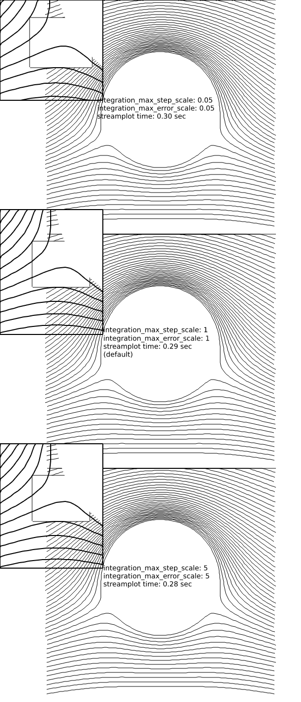
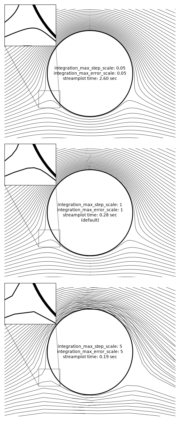
images_contours_and_fields/quadmesh_demo
=============
Source
"""
=============
QuadMesh Demo
=============

`~.axes.Axes.pcolormesh` uses a `~matplotlib.collections.QuadMesh`,
a faster generalization of `~.axes.Axes.pcolor`, but with some restrictions.

This demo illustrates a bug in quadmesh with masked data.
"""

import numpy as np

from matplotlib import pyplot as plt

n = 12
x = np.linspace(-1.5, 1.5, n)
y = np.linspace(-1.5, 1.5, n * 2)
X, Y = np.meshgrid(x, y)
Qx = np.cos(Y) - np.cos(X)
Qz = np.sin(Y) + np.sin(X)
Z = np.sqrt(X**2 + Y**2) / 5
Z = (Z - Z.min()) / (Z.max() - Z.min())

# The color array can include masked values.
Zm = np.ma.masked_where(np.abs(Qz) < 0.5 * np.max(Qz), Z)

fig, axs = plt.subplots(nrows=1, ncols=3)
axs[0].pcolormesh(Qx, Qz, Z, shading='gouraud')
axs[0].set_title('Without masked values')

# You can control the color of the masked region.
cmap = plt.colormaps[plt.rcParams['image.cmap']].with_extremes(bad='y')
axs[1].pcolormesh(Qx, Qz, Zm, shading='gouraud', cmap=cmap)
axs[1].set_title('With masked values')

# Or use the default, which is transparent.
axs[2].pcolormesh(Qx, Qz, Zm, shading='gouraud')
axs[2].set_title('With masked values')

fig.tight_layout()
plt.show()

# %%
#
# .. admonition:: References
#
#    The use of the following functions, methods, classes and modules is shown
#    in this example:
#
#    - `matplotlib.axes.Axes.pcolormesh` / `matplotlib.pyplot.pcolormesh`
images_contours_and_fields/quiver_demo
=======================================
Source
"""
=======================================
Advanced quiver and quiverkey functions
=======================================

Demonstrates some more advanced options for `~.axes.Axes.quiver`.  For a simple
example refer to :doc:`/gallery/images_contours_and_fields/quiver_simple_demo`.

Note: The plot autoscaling does not take into account the arrows, so
those on the boundaries may reach out of the picture.  This is not an easy
problem to solve in a perfectly general way.  The recommended workaround is to
manually set the Axes limits in such a case.
"""

import matplotlib.pyplot as plt
import numpy as np

X, Y = np.meshgrid(np.arange(0, 2 * np.pi, .2), np.arange(0, 2 * np.pi, .2))
U = np.cos(X)
V = np.sin(Y)

# %%

fig1, ax1 = plt.subplots()
ax1.set_title('Arrows scale with plot width, not view')
Q = ax1.quiver(X, Y, U, V, units='width')
qk = ax1.quiverkey(Q, 0.9, 0.9, 2, r'$2 \frac{m}{s}$', labelpos='E',
                   coordinates='figure')

# %%

fig2, ax2 = plt.subplots()
ax2.set_title("pivot='middle'; every third arrow; units='inches'")
Q = ax2.quiver(X[::3, ::3], Y[::3, ::3], U[::3, ::3], V[::3, ::3],
               pivot='middle', units='inches')
qk = ax2.quiverkey(Q, 0.9, 0.9, 1, r'$1 \frac{m}{s}$', labelpos='E',
                   coordinates='figure')
ax2.scatter(X[::3, ::3], Y[::3, ::3], color='r', s=5)

# %%

# sphinx_gallery_thumbnail_number = 3

fig3, ax3 = plt.subplots()
ax3.set_title("pivot='tip'; scales with x view")
M = np.hypot(U, V)
Q = ax3.quiver(X, Y, U, V, M, units='x', pivot='tip', width=0.022,
               scale=1 / 0.15)
qk = ax3.quiverkey(Q, 0.9, 0.9, 1, r'$1 \frac{m}{s}$', labelpos='E',
                   coordinates='figure')
ax3.scatter(X, Y, color='0.5', s=1)

plt.show()

# %%
#
# .. admonition:: References
#
#    The use of the following functions, methods, classes and modules is shown
#    in this example:
#
#    - `matplotlib.axes.Axes.quiver` / `matplotlib.pyplot.quiver`
#    - `matplotlib.axes.Axes.quiverkey` / `matplotlib.pyplot.quiverkey`
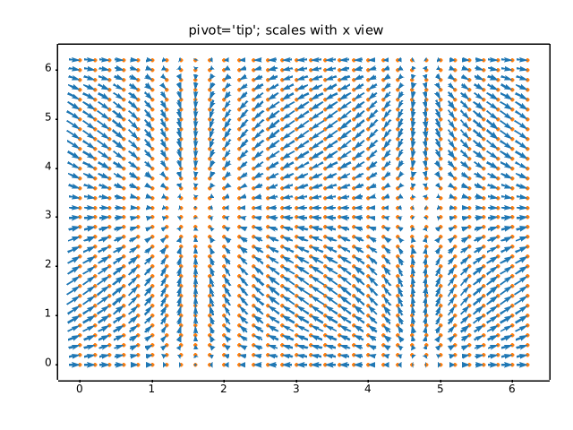
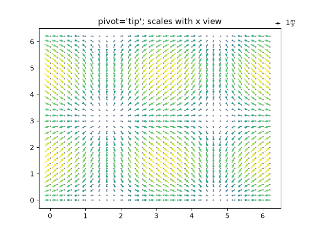
images_contours_and_fields/quiver_simple_demo
==================
Source
"""
==================
Quiver Simple Demo
==================

A simple example of a `~.axes.Axes.quiver` plot with a `~.axes.Axes.quiverkey`.

For more advanced options refer to
:doc:`/gallery/images_contours_and_fields/quiver_demo`.
"""
import matplotlib.pyplot as plt
import numpy as np

X = np.arange(-10, 10, 1)
Y = np.arange(-10, 10, 1)
U, V = np.meshgrid(X, Y)

fig, ax = plt.subplots()
q = ax.quiver(X, Y, U, V)
ax.quiverkey(q, X=0.3, Y=1.1, U=10,
             label='Quiver key, length = 10', labelpos='E')

plt.show()

# %%
#
# .. admonition:: References
#
#    The use of the following functions, methods, classes and modules is shown
#    in this example:
#
#    - `matplotlib.axes.Axes.quiver` / `matplotlib.pyplot.quiver`
#    - `matplotlib.axes.Axes.quiverkey` / `matplotlib.pyplot.quiverkey`
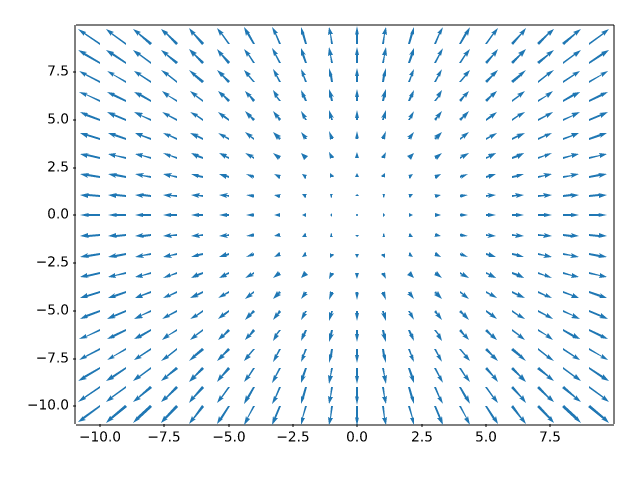
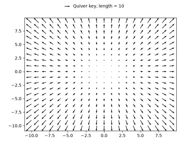
images_contours_and_fields/shading_example
===============
Source
"""
===============
Shading example
===============

Example showing how to make shaded relief plots like Mathematica_ or
`Generic Mapping Tools`_.

.. _Mathematica: http://reference.wolfram.com/mathematica/ref/ReliefPlot.html
.. _Generic Mapping Tools: https://www.generic-mapping-tools.org/
"""

import matplotlib.pyplot as plt
import numpy as np

from matplotlib import cbook
from matplotlib.colors import LightSource


def main():
    # Test data
    x, y = np.mgrid[-5:5:0.05, -5:5:0.05]
    z = 5 * (np.sqrt(x**2 + y**2) + np.sin(x**2 + y**2))

    dem = cbook.get_sample_data('jacksboro_fault_dem.npz')
    elev = dem['elevation']

    fig = compare(z, plt.colormaps["copper"])
    fig.suptitle('HSV Blending Looks Best with Smooth Surfaces', y=0.95)

    fig = compare(elev, plt.colormaps["gist_earth"], ve=0.05)
    fig.suptitle('Overlay Blending Looks Best with Rough Surfaces', y=0.95)

    plt.show()


def compare(z, cmap, ve=1):
    # Create subplots and hide ticks
    fig, axs = plt.subplots(ncols=2, nrows=2)
    for ax in axs.flat:
        ax.set(xticks=[], yticks=[])

    # Illuminate the scene from the northwest
    ls = LightSource(azdeg=315, altdeg=45)

    axs[0, 0].imshow(z, cmap=cmap)
    axs[0, 0].set(xlabel='Colormapped Data')

    axs[0, 1].imshow(ls.hillshade(z, vert_exag=ve), cmap='gray')
    axs[0, 1].set(xlabel='Illumination Intensity')

    rgb = ls.shade(z, cmap=cmap, vert_exag=ve, blend_mode='hsv')
    axs[1, 0].imshow(rgb)
    axs[1, 0].set(xlabel='Blend Mode: "hsv" (default)')

    rgb = ls.shade(z, cmap=cmap, vert_exag=ve, blend_mode='overlay')
    axs[1, 1].imshow(rgb)
    axs[1, 1].set(xlabel='Blend Mode: "overlay"')

    return fig


if __name__ == '__main__':
    main()

# %%
#
# .. admonition:: References
#
#    The use of the following functions, methods, classes and modules is shown
#    in this example:
#
#    - `matplotlib.colors.LightSource`
#    - `matplotlib.axes.Axes.imshow` / `matplotlib.pyplot.imshow`
images_contours_and_fields/specgram_demo
===========
Source
"""
===========
Spectrogram
===========

Plotting a spectrogram using `~.Axes.specgram`.
"""
import matplotlib.pyplot as plt
import numpy as np

# Fixing random state for reproducibility
np.random.seed(19680801)

dt = 0.0005
t = np.arange(0.0, 20.5, dt)
s1 = np.sin(2 * np.pi * 100 * t)
s2 = 2 * np.sin(2 * np.pi * 400 * t)

# create a transient "chirp"
s2[t <= 10] = s2[12 <= t] = 0

# add some noise into the mix
nse = 0.01 * np.random.random(size=len(t))

x = s1 + s2 + nse  # the signal
NFFT = 1024  # the length of the windowing segments
Fs = 1/dt  # the sampling frequency

fig, (ax1, ax2) = plt.subplots(nrows=2, sharex=True)
ax1.plot(t, x)
ax1.set_ylabel('Signal')

Pxx, freqs, bins, im = ax2.specgram(x, NFFT=NFFT, Fs=Fs)
# The `specgram` method returns 4 objects. They are:
# - Pxx: the periodogram
# - freqs: the frequency vector
# - bins: the centers of the time bins
# - im: the .image.AxesImage instance representing the data in the plot
ax2.set_xlabel('Time (s)')
ax2.set_ylabel('Frequency (Hz)')
ax2.set_xlim(0, 20)

plt.show()

# %%
#
# .. admonition:: References
#
#    The use of the following functions, methods, classes and modules is shown
#    in this example:
#
#    - `matplotlib.axes.Axes.specgram` / `matplotlib.pyplot.specgram`
images_contours_and_fields/spy_demos
=========
Source
"""
=========
Spy Demos
=========

Plot the sparsity pattern of arrays.
"""

import matplotlib.pyplot as plt
import numpy as np

# Fixing random state for reproducibility
np.random.seed(19680801)

fig, axs = plt.subplots(2, 2)
ax1 = axs[0, 0]
ax2 = axs[0, 1]
ax3 = axs[1, 0]
ax4 = axs[1, 1]

x = np.random.randn(20, 20)
x[5, :] = 0.
x[:, 12] = 0.

ax1.spy(x, markersize=5)
ax2.spy(x, precision=0.1, markersize=5)

ax3.spy(x)
ax4.spy(x, precision=0.1)

plt.show()

# %%
#
# .. admonition:: References
#
#    The use of the following functions, methods, classes and modules is shown
#    in this example:
#
#    - `matplotlib.axes.Axes.spy` / `matplotlib.pyplot.spy`
images_contours_and_fields/tricontour_demo
===============
Source
"""
===============
Tricontour Demo
===============

Contour plots of unstructured triangular grids.
"""
import matplotlib.pyplot as plt
import numpy as np

import matplotlib.tri as tri

# %%
# Creating a Triangulation without specifying the triangles results in the
# Delaunay triangulation of the points.

# First create the x and y coordinates of the points.
n_angles = 48
n_radii = 8
min_radius = 0.25
radii = np.linspace(min_radius, 0.95, n_radii)

angles = np.linspace(0, 2 * np.pi, n_angles, endpoint=False)
angles = np.repeat(angles[..., np.newaxis], n_radii, axis=1)
angles[:, 1::2] += np.pi / n_angles

x = (radii * np.cos(angles)).flatten()
y = (radii * np.sin(angles)).flatten()
z = (np.cos(radii) * np.cos(3 * angles)).flatten()

# Create the Triangulation; no triangles so Delaunay triangulation created.
triang = tri.Triangulation(x, y)

# Mask off unwanted triangles.
triang.set_mask(np.hypot(x[triang.triangles].mean(axis=1),
                         y[triang.triangles].mean(axis=1))
                < min_radius)

# %%
# pcolor plot.

fig1, ax1 = plt.subplots()
ax1.set_aspect('equal')
tcf = ax1.tricontourf(triang, z)
fig1.colorbar(tcf)
ax1.tricontour(triang, z, colors='k')
ax1.set_title('Contour plot of Delaunay triangulation')


# %%
# You could also specify hatching patterns along with different cmaps.

fig2, ax2 = plt.subplots()
ax2.set_aspect("equal")
tcf = ax2.tricontourf(
    triang,
    z,
    hatches=["*", "-", "/", "//", "\\", None],
    cmap="cividis"
)
fig2.colorbar(tcf)
ax2.tricontour(triang, z, linestyles="solid", colors="k", linewidths=2.0)
ax2.set_title("Hatched Contour plot of Delaunay triangulation")

# %%
# You could also generate hatching patterns labeled with no color.

fig3, ax3 = plt.subplots()
n_levels = 7
tcf = ax3.tricontourf(
    triang,
    z,
    n_levels,
    colors="none",
    hatches=[".", "/", "\\", None, "\\\\", "*"],
)
ax3.tricontour(triang, z, n_levels, colors="black", linestyles="-")


# create a legend for the contour set
artists, labels = tcf.legend_elements(str_format="{:2.1f}".format)
ax3.legend(artists, labels, handleheight=2, framealpha=1)

# %%
# You can specify your own triangulation rather than perform a Delaunay
# triangulation of the points, where each triangle is given by the indices of
# the three points that make up the triangle, ordered in either a clockwise or
# anticlockwise manner.

xy = np.asarray([
    [-0.101, 0.872], [-0.080, 0.883], [-0.069, 0.888], [-0.054, 0.890],
    [-0.045, 0.897], [-0.057, 0.895], [-0.073, 0.900], [-0.087, 0.898],
    [-0.090, 0.904], [-0.069, 0.907], [-0.069, 0.921], [-0.080, 0.919],
    [-0.073, 0.928], [-0.052, 0.930], [-0.048, 0.942], [-0.062, 0.949],
    [-0.054, 0.958], [-0.069, 0.954], [-0.087, 0.952], [-0.087, 0.959],
    [-0.080, 0.966], [-0.085, 0.973], [-0.087, 0.965], [-0.097, 0.965],
    [-0.097, 0.975], [-0.092, 0.984], [-0.101, 0.980], [-0.108, 0.980],
    [-0.104, 0.987], [-0.102, 0.993], [-0.115, 1.001], [-0.099, 0.996],
    [-0.101, 1.007], [-0.090, 1.010], [-0.087, 1.021], [-0.069, 1.021],
    [-0.052, 1.022], [-0.052, 1.017], [-0.069, 1.010], [-0.064, 1.005],
    [-0.048, 1.005], [-0.031, 1.005], [-0.031, 0.996], [-0.040, 0.987],
    [-0.045, 0.980], [-0.052, 0.975], [-0.040, 0.973], [-0.026, 0.968],
    [-0.020, 0.954], [-0.006, 0.947], [ 0.003, 0.935], [ 0.006, 0.926],
    [ 0.005, 0.921], [ 0.022, 0.923], [ 0.033, 0.912], [ 0.029, 0.905],
    [ 0.017, 0.900], [ 0.012, 0.895], [ 0.027, 0.893], [ 0.019, 0.886],
    [ 0.001, 0.883], [-0.012, 0.884], [-0.029, 0.883], [-0.038, 0.879],
    [-0.057, 0.881], [-0.062, 0.876], [-0.078, 0.876], [-0.087, 0.872],
    [-0.030, 0.907], [-0.007, 0.905], [-0.057, 0.916], [-0.025, 0.933],
    [-0.077, 0.990], [-0.059, 0.993]])
x = np.degrees(xy[:, 0])
y = np.degrees(xy[:, 1])
x0 = -5
y0 = 52
z = np.exp(-0.01 * ((x - x0) ** 2 + (y - y0) ** 2))

triangles = np.asarray([
    [67, 66,  1], [65,  2, 66], [ 1, 66,  2], [64,  2, 65], [63,  3, 64],
    [60, 59, 57], [ 2, 64,  3], [ 3, 63,  4], [ 0, 67,  1], [62,  4, 63],
    [57, 59, 56], [59, 58, 56], [61, 60, 69], [57, 69, 60], [ 4, 62, 68],
    [ 6,  5,  9], [61, 68, 62], [69, 68, 61], [ 9,  5, 70], [ 6,  8,  7],
    [ 4, 70,  5], [ 8,  6,  9], [56, 69, 57], [69, 56, 52], [70, 10,  9],
    [54, 53, 55], [56, 55, 53], [68, 70,  4], [52, 56, 53], [11, 10, 12],
    [69, 71, 68], [68, 13, 70], [10, 70, 13], [51, 50, 52], [13, 68, 71],
    [52, 71, 69], [12, 10, 13], [71, 52, 50], [71, 14, 13], [50, 49, 71],
    [49, 48, 71], [14, 16, 15], [14, 71, 48], [17, 19, 18], [17, 20, 19],
    [48, 16, 14], [48, 47, 16], [47, 46, 16], [16, 46, 45], [23, 22, 24],
    [21, 24, 22], [17, 16, 45], [20, 17, 45], [21, 25, 24], [27, 26, 28],
    [20, 72, 21], [25, 21, 72], [45, 72, 20], [25, 28, 26], [44, 73, 45],
    [72, 45, 73], [28, 25, 29], [29, 25, 31], [43, 73, 44], [73, 43, 40],
    [72, 73, 39], [72, 31, 25], [42, 40, 43], [31, 30, 29], [39, 73, 40],
    [42, 41, 40], [72, 33, 31], [32, 31, 33], [39, 38, 72], [33, 72, 38],
    [33, 38, 34], [37, 35, 38], [34, 38, 35], [35, 37, 36]])

# %%
# Rather than create a Triangulation object, can simply pass x, y and triangles
# arrays to tripcolor directly.  It would be better to use a Triangulation
# object if the same triangulation was to be used more than once to save
# duplicated calculations.

fig4, ax4 = plt.subplots()
ax4.set_aspect('equal')
tcf = ax4.tricontourf(x, y, triangles, z)
fig4.colorbar(tcf)
ax4.set_title('Contour plot of user-specified triangulation')
ax4.set_xlabel('Longitude (degrees)')
ax4.set_ylabel('Latitude (degrees)')

plt.show()

# %%
#
# .. admonition:: References
#
#    The use of the following functions, methods, classes and modules is shown
#    in this example:
#
#    - `matplotlib.axes.Axes.tricontourf` / `matplotlib.pyplot.tricontourf`
#    - `matplotlib.tri.Triangulation`
#    - `matplotlib.figure.Figure.colorbar` / `matplotlib.pyplot.colorbar`
#    - `matplotlib.axes.Axes.legend` / `matplotlib.pyplot.legend`
#    - `matplotlib.contour.ContourSet.legend_elements`
images_contours_and_fields/tricontour_smooth_delaunay
==========================
Source
"""
==========================
Tricontour Smooth Delaunay
==========================

Demonstrates high-resolution tricontouring of a random set of points;
a `matplotlib.tri.TriAnalyzer` is used to improve the plot quality.

The initial data points and triangular grid for this demo are:

- a set of random points is instantiated, inside [-1, 1] x [-1, 1] square
- A Delaunay triangulation of these points is then computed, of which a
  random subset of triangles is masked out by the user (based on
  *init_mask_frac* parameter). This simulates invalidated data.

The proposed generic procedure to obtain a high resolution contouring of such
a data set is the following:

1. Compute an extended mask with a `matplotlib.tri.TriAnalyzer`, which will
   exclude badly shaped (flat) triangles from the border of the
   triangulation. Apply the mask to the triangulation (using set_mask).
2. Refine and interpolate the data using a `matplotlib.tri.UniformTriRefiner`.
3. Plot the refined data with `~.axes.Axes.tricontour`.

"""
import matplotlib.pyplot as plt
import numpy as np

from matplotlib.tri import TriAnalyzer, Triangulation, UniformTriRefiner


# ----------------------------------------------------------------------------
# Analytical test function
# ----------------------------------------------------------------------------
def experiment_res(x, y):
    """An analytic function representing experiment results."""
    x = 2 * x
    r1 = np.sqrt((0.5 - x)**2 + (0.5 - y)**2)
    theta1 = np.arctan2(0.5 - x, 0.5 - y)
    r2 = np.sqrt((-x - 0.2)**2 + (-y - 0.2)**2)
    theta2 = np.arctan2(-x - 0.2, -y - 0.2)
    z = (4 * (np.exp((r1/10)**2) - 1) * 30 * np.cos(3 * theta1) +
         (np.exp((r2/10)**2) - 1) * 30 * np.cos(5 * theta2) +
         2 * (x**2 + y**2))
    return (np.max(z) - z) / (np.max(z) - np.min(z))

# ----------------------------------------------------------------------------
# Generating the initial data test points and triangulation for the demo
# ----------------------------------------------------------------------------
# User parameters for data test points

# Number of test data points, tested from 3 to 5000 for subdiv=3
n_test = 200

# Number of recursive subdivisions of the initial mesh for smooth plots.
# Values >3 might result in a very high number of triangles for the refine
# mesh: new triangles numbering = (4**subdiv)*ntri
subdiv = 3

# Float > 0. adjusting the proportion of (invalid) initial triangles which will
# be masked out. Enter 0 for no mask.
init_mask_frac = 0.0

# Minimum circle ratio - border triangles with circle ratio below this will be
# masked if they touch a border. Suggested value 0.01; use -1 to keep all
# triangles.
min_circle_ratio = .01

# Random points
random_gen = np.random.RandomState(seed=19680801)
x_test = random_gen.uniform(-1., 1., size=n_test)
y_test = random_gen.uniform(-1., 1., size=n_test)
z_test = experiment_res(x_test, y_test)

# meshing with Delaunay triangulation
tri = Triangulation(x_test, y_test)
ntri = tri.triangles.shape[0]

# Some invalid data are masked out
mask_init = np.zeros(ntri, dtype=bool)
masked_tri = random_gen.randint(0, ntri, int(ntri * init_mask_frac))
mask_init[masked_tri] = True
tri.set_mask(mask_init)


# ----------------------------------------------------------------------------
# Improving the triangulation before high-res plots: removing flat triangles
# ----------------------------------------------------------------------------
# masking badly shaped triangles at the border of the triangular mesh.
mask = TriAnalyzer(tri).get_flat_tri_mask(min_circle_ratio)
tri.set_mask(mask)

# refining the data
refiner = UniformTriRefiner(tri)
tri_refi, z_test_refi = refiner.refine_field(z_test, subdiv=subdiv)

# analytical 'results' for comparison
z_expected = experiment_res(tri_refi.x, tri_refi.y)

# for the demo: loading the 'flat' triangles for plot
flat_tri = Triangulation(x_test, y_test)
flat_tri.set_mask(~mask)


# ----------------------------------------------------------------------------
# Now the plots
# ----------------------------------------------------------------------------
# User options for plots
plot_tri = True          # plot of base triangulation
plot_masked_tri = True   # plot of excessively flat excluded triangles
plot_refi_tri = False    # plot of refined triangulation
plot_expected = False    # plot of analytical function values for comparison


# Graphical options for tricontouring
levels = np.arange(0., 1., 0.025)

fig, ax = plt.subplots()
ax.set_aspect('equal')
ax.set_title("Filtering a Delaunay mesh\n"
             "(application to high-resolution tricontouring)")

# 1) plot of the refined (computed) data contours:
ax.tricontour(tri_refi, z_test_refi, levels=levels, cmap='Blues',
              linewidths=[2.0, 0.5, 1.0, 0.5])
# 2) plot of the expected (analytical) data contours (dashed):
if plot_expected:
    ax.tricontour(tri_refi, z_expected, levels=levels, cmap='Blues',
                  linestyles='--')
# 3) plot of the fine mesh on which interpolation was done:
if plot_refi_tri:
    ax.triplot(tri_refi, color='0.97')
# 4) plot of the initial 'coarse' mesh:
if plot_tri:
    ax.triplot(tri, color='0.7')
# 4) plot of the unvalidated triangles from naive Delaunay Triangulation:
if plot_masked_tri:
    ax.triplot(flat_tri, color='red')

plt.show()

# %%
#
# .. admonition:: References
#
#    The use of the following functions, methods, classes and modules is shown
#    in this example:
#
#    - `matplotlib.axes.Axes.tricontour` / `matplotlib.pyplot.tricontour`
#    - `matplotlib.axes.Axes.tricontourf` / `matplotlib.pyplot.tricontourf`
#    - `matplotlib.axes.Axes.triplot` / `matplotlib.pyplot.triplot`
#    - `matplotlib.tri`
#    - `matplotlib.tri.Triangulation`
#    - `matplotlib.tri.TriAnalyzer`
#    - `matplotlib.tri.UniformTriRefiner`
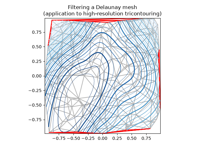
images_contours_and_fields/tricontour_smooth_user
======================
Source
"""
======================
Tricontour Smooth User
======================

Demonstrates high-resolution tricontouring on user-defined triangular grids
with `matplotlib.tri.UniformTriRefiner`.
"""
import matplotlib.pyplot as plt
import numpy as np

import matplotlib.tri as tri


# ----------------------------------------------------------------------------
# Analytical test function
# ----------------------------------------------------------------------------
def function_z(x, y):
    r1 = np.sqrt((0.5 - x)**2 + (0.5 - y)**2)
    theta1 = np.arctan2(0.5 - x, 0.5 - y)
    r2 = np.sqrt((-x - 0.2)**2 + (-y - 0.2)**2)
    theta2 = np.arctan2(-x - 0.2, -y - 0.2)
    z = -(2 * (np.exp((r1 / 10)**2) - 1) * 30. * np.cos(7. * theta1) +
          (np.exp((r2 / 10)**2) - 1) * 30. * np.cos(11. * theta2) +
          0.7 * (x**2 + y**2))
    return (np.max(z) - z) / (np.max(z) - np.min(z))

# ----------------------------------------------------------------------------
# Creating a Triangulation
# ----------------------------------------------------------------------------
# First create the x and y coordinates of the points.
n_angles = 20
n_radii = 10
min_radius = 0.15
radii = np.linspace(min_radius, 0.95, n_radii)

angles = np.linspace(0, 2 * np.pi, n_angles, endpoint=False)
angles = np.repeat(angles[..., np.newaxis], n_radii, axis=1)
angles[:, 1::2] += np.pi / n_angles

x = (radii * np.cos(angles)).flatten()
y = (radii * np.sin(angles)).flatten()
z = function_z(x, y)

# Now create the Triangulation.
# (Creating a Triangulation without specifying the triangles results in the
# Delaunay triangulation of the points.)
triang = tri.Triangulation(x, y)

# Mask off unwanted triangles.
triang.set_mask(np.hypot(x[triang.triangles].mean(axis=1),
                         y[triang.triangles].mean(axis=1))
                < min_radius)

# ----------------------------------------------------------------------------
# Refine data
# ----------------------------------------------------------------------------
refiner = tri.UniformTriRefiner(triang)
tri_refi, z_test_refi = refiner.refine_field(z, subdiv=3)

# ----------------------------------------------------------------------------
# Plot the triangulation and the high-res iso-contours
# ----------------------------------------------------------------------------
fig, ax = plt.subplots()
ax.set_aspect('equal')
ax.triplot(triang, lw=0.5, color='white')

levels = np.arange(0., 1., 0.025)
ax.tricontourf(tri_refi, z_test_refi, levels=levels, cmap='terrain')
ax.tricontour(tri_refi, z_test_refi, levels=levels,
              colors=['0.25', '0.5', '0.5', '0.5', '0.5'],
              linewidths=[1.0, 0.5, 0.5, 0.5, 0.5])

ax.set_title("High-resolution tricontouring")

plt.show()

# %%
#
# .. admonition:: References
#
#    The use of the following functions, methods, classes and modules is shown
#    in this example:
#
#    - `matplotlib.axes.Axes.tricontour` / `matplotlib.pyplot.tricontour`
#    - `matplotlib.axes.Axes.tricontourf` / `matplotlib.pyplot.tricontourf`
#    - `matplotlib.tri`
#    - `matplotlib.tri.Triangulation`
#    - `matplotlib.tri.UniformTriRefiner`
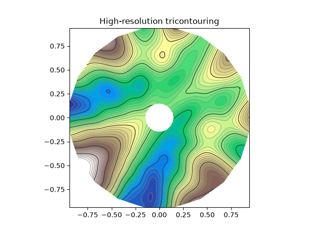
images_contours_and_fields/trigradient_demo
================
Source
"""
================
Trigradient Demo
================

Demonstrates computation of gradient with
`matplotlib.tri.CubicTriInterpolator`.
"""
import matplotlib.pyplot as plt
import numpy as np

from matplotlib.tri import CubicTriInterpolator, Triangulation, UniformTriRefiner


# ----------------------------------------------------------------------------
# Electrical potential of a dipole
# ----------------------------------------------------------------------------
def dipole_potential(x, y):
    """The electric dipole potential V, at position *x*, *y*."""
    r_sq = x**2 + y**2
    theta = np.arctan2(y, x)
    z = np.cos(theta)/r_sq
    return (np.max(z) - z) / (np.max(z) - np.min(z))


# ----------------------------------------------------------------------------
# Creating a Triangulation
# ----------------------------------------------------------------------------
# First create the x and y coordinates of the points.
n_angles = 30
n_radii = 10
min_radius = 0.2
radii = np.linspace(min_radius, 0.95, n_radii)

angles = np.linspace(0, 2 * np.pi, n_angles, endpoint=False)
angles = np.repeat(angles[..., np.newaxis], n_radii, axis=1)
angles[:, 1::2] += np.pi / n_angles

x = (radii*np.cos(angles)).flatten()
y = (radii*np.sin(angles)).flatten()
V = dipole_potential(x, y)

# Create the Triangulation; no triangles specified so Delaunay triangulation
# created.
triang = Triangulation(x, y)

# Mask off unwanted triangles.
triang.set_mask(np.hypot(x[triang.triangles].mean(axis=1),
                         y[triang.triangles].mean(axis=1))
                < min_radius)

# ----------------------------------------------------------------------------
# Refine data - interpolates the electrical potential V
# ----------------------------------------------------------------------------
refiner = UniformTriRefiner(triang)
tri_refi, z_test_refi = refiner.refine_field(V, subdiv=3)

# ----------------------------------------------------------------------------
# Computes the electrical field (Ex, Ey) as gradient of electrical potential
# ----------------------------------------------------------------------------
tci = CubicTriInterpolator(triang, -V)
# Gradient requested here at the mesh nodes but could be anywhere else:
(Ex, Ey) = tci.gradient(triang.x, triang.y)
E_norm = np.sqrt(Ex**2 + Ey**2)

# ----------------------------------------------------------------------------
# Plot the triangulation, the potential iso-contours and the vector field
# ----------------------------------------------------------------------------
fig, ax = plt.subplots()
ax.set_aspect('equal')
# Enforce the margins, and enlarge them to give room for the vectors.
ax.use_sticky_edges = False
ax.margins(0.07)

ax.triplot(triang, color='0.8')

levels = np.arange(0., 1., 0.01)
ax.tricontour(tri_refi, z_test_refi, levels=levels, cmap='hot',
              linewidths=[2.0, 1.0, 1.0, 1.0])
# Plots direction of the electrical vector field
ax.quiver(triang.x, triang.y, Ex/E_norm, Ey/E_norm,
          units='xy', scale=10., zorder=3, color='blue',
          width=0.007, headwidth=3., headlength=4.)

ax.set_title('Gradient plot: an electrical dipole')
plt.show()

# %%
#
# .. admonition:: References
#
#    The use of the following functions, methods, classes and modules is shown
#    in this example:
#
#    - `matplotlib.axes.Axes.tricontour` / `matplotlib.pyplot.tricontour`
#    - `matplotlib.axes.Axes.triplot` / `matplotlib.pyplot.triplot`
#    - `matplotlib.tri`
#    - `matplotlib.tri.Triangulation`
#    - `matplotlib.tri.CubicTriInterpolator`
#    - `matplotlib.tri.CubicTriInterpolator.gradient`
#    - `matplotlib.tri.UniformTriRefiner`
#    - `matplotlib.axes.Axes.quiver` / `matplotlib.pyplot.quiver`
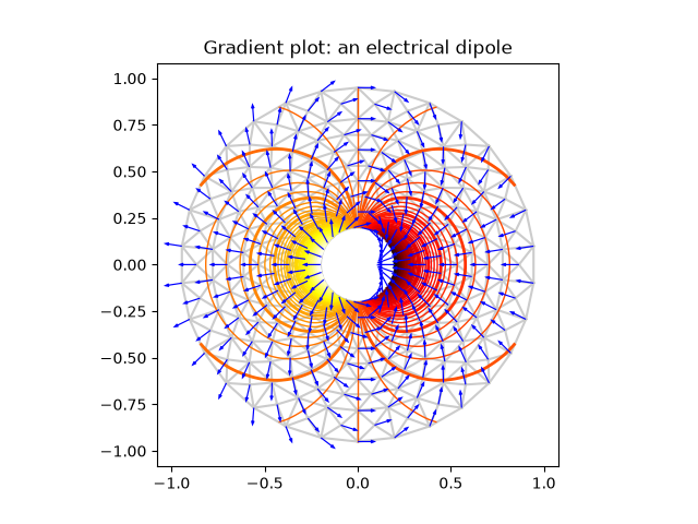
images_contours_and_fields/triinterp_demo
==============
Source
"""
==============
Triinterp Demo
==============

Interpolation from triangular grid to quad grid.
"""
import matplotlib.pyplot as plt
import numpy as np

import matplotlib.tri as mtri

# Create triangulation.
x = np.asarray([0, 1, 2, 3, 0.5, 1.5, 2.5, 1, 2, 1.5])
y = np.asarray([0, 0, 0, 0, 1.0, 1.0, 1.0, 2, 2, 3.0])
triangles = [[0, 1, 4], [1, 2, 5], [2, 3, 6], [1, 5, 4], [2, 6, 5], [4, 5, 7],
             [5, 6, 8], [5, 8, 7], [7, 8, 9]]
triang = mtri.Triangulation(x, y, triangles)

# Interpolate to regularly-spaced quad grid.
z = np.cos(1.5 * x) * np.cos(1.5 * y)
xi, yi = np.meshgrid(np.linspace(0, 3, 20), np.linspace(0, 3, 20))

interp_lin = mtri.LinearTriInterpolator(triang, z)
zi_lin = interp_lin(xi, yi)

interp_cubic_geom = mtri.CubicTriInterpolator(triang, z, kind='geom')
zi_cubic_geom = interp_cubic_geom(xi, yi)

interp_cubic_min_E = mtri.CubicTriInterpolator(triang, z, kind='min_E')
zi_cubic_min_E = interp_cubic_min_E(xi, yi)

# Set up the figure
fig, axs = plt.subplots(nrows=2, ncols=2)
axs = axs.flatten()

# Plot the triangulation.
axs[0].tricontourf(triang, z)
axs[0].triplot(triang, 'ko-')
axs[0].set_title('Triangular grid')

# Plot linear interpolation to quad grid.
axs[1].contourf(xi, yi, zi_lin)
axs[1].plot(xi, yi, 'k-', lw=0.5, alpha=0.5)
axs[1].plot(xi.T, yi.T, 'k-', lw=0.5, alpha=0.5)
axs[1].set_title("Linear interpolation")

# Plot cubic interpolation to quad grid, kind=geom
axs[2].contourf(xi, yi, zi_cubic_geom)
axs[2].plot(xi, yi, 'k-', lw=0.5, alpha=0.5)
axs[2].plot(xi.T, yi.T, 'k-', lw=0.5, alpha=0.5)
axs[2].set_title("Cubic interpolation,\nkind='geom'")

# Plot cubic interpolation to quad grid, kind=min_E
axs[3].contourf(xi, yi, zi_cubic_min_E)
axs[3].plot(xi, yi, 'k-', lw=0.5, alpha=0.5)
axs[3].plot(xi.T, yi.T, 'k-', lw=0.5, alpha=0.5)
axs[3].set_title("Cubic interpolation,\nkind='min_E'")

fig.tight_layout()
plt.show()

# %%
#
# .. admonition:: References
#
#    The use of the following functions, methods, classes and modules is shown
#    in this example:
#
#    - `matplotlib.axes.Axes.tricontourf` / `matplotlib.pyplot.tricontourf`
#    - `matplotlib.axes.Axes.triplot` / `matplotlib.pyplot.triplot`
#    - `matplotlib.axes.Axes.contourf` / `matplotlib.pyplot.contourf`
#    - `matplotlib.axes.Axes.plot` / `matplotlib.pyplot.plot`
#    - `matplotlib.tri`
#    - `matplotlib.tri.LinearTriInterpolator`
#    - `matplotlib.tri.CubicTriInterpolator`
#    - `matplotlib.tri.Triangulation`
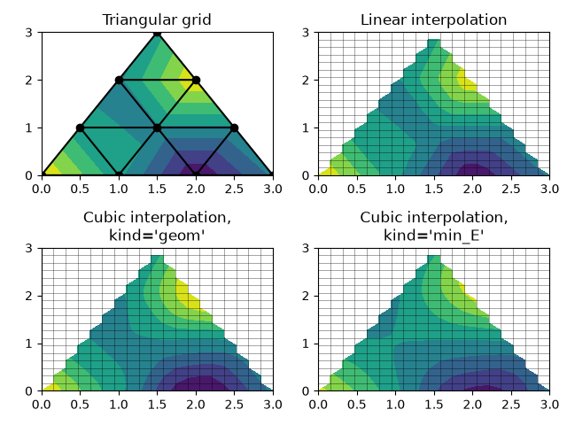
images_contours_and_fields/tripcolor_demo
==============
Source
"""
==============
Tripcolor Demo
==============

Pseudocolor plots of unstructured triangular grids.
"""
import matplotlib.pyplot as plt
import numpy as np

import matplotlib.tri as tri

# %%
# Creating a Triangulation without specifying the triangles results in the
# Delaunay triangulation of the points.

# First create the x and y coordinates of the points.
n_angles = 36
n_radii = 8
min_radius = 0.25
radii = np.linspace(min_radius, 0.95, n_radii)

angles = np.linspace(0, 2 * np.pi, n_angles, endpoint=False)
angles = np.repeat(angles[..., np.newaxis], n_radii, axis=1)
angles[:, 1::2] += np.pi / n_angles

x = (radii * np.cos(angles)).flatten()
y = (radii * np.sin(angles)).flatten()
z = (np.cos(radii) * np.cos(3 * angles)).flatten()

# Create the Triangulation; no triangles so Delaunay triangulation created.
triang = tri.Triangulation(x, y)

# Mask off unwanted triangles.
triang.set_mask(np.hypot(x[triang.triangles].mean(axis=1),
                         y[triang.triangles].mean(axis=1))
                < min_radius)

# %%
# tripcolor plot.

fig1, ax1 = plt.subplots()
ax1.set_aspect('equal')
tpc = ax1.tripcolor(triang, z, shading='flat')
fig1.colorbar(tpc)
ax1.set_title('tripcolor of Delaunay triangulation, flat shading')

# %%
# Illustrate Gouraud shading.

fig2, ax2 = plt.subplots()
ax2.set_aspect('equal')
tpc = ax2.tripcolor(triang, z, shading='gouraud')
fig2.colorbar(tpc)
ax2.set_title('tripcolor of Delaunay triangulation, gouraud shading')


# %%
# You can specify your own triangulation rather than perform a Delaunay
# triangulation of the points, where each triangle is given by the indices of
# the three points that make up the triangle, ordered in either a clockwise or
# anticlockwise manner.

xy = np.asarray([
    [-0.101, 0.872], [-0.080, 0.883], [-0.069, 0.888], [-0.054, 0.890],
    [-0.045, 0.897], [-0.057, 0.895], [-0.073, 0.900], [-0.087, 0.898],
    [-0.090, 0.904], [-0.069, 0.907], [-0.069, 0.921], [-0.080, 0.919],
    [-0.073, 0.928], [-0.052, 0.930], [-0.048, 0.942], [-0.062, 0.949],
    [-0.054, 0.958], [-0.069, 0.954], [-0.087, 0.952], [-0.087, 0.959],
    [-0.080, 0.966], [-0.085, 0.973], [-0.087, 0.965], [-0.097, 0.965],
    [-0.097, 0.975], [-0.092, 0.984], [-0.101, 0.980], [-0.108, 0.980],
    [-0.104, 0.987], [-0.102, 0.993], [-0.115, 1.001], [-0.099, 0.996],
    [-0.101, 1.007], [-0.090, 1.010], [-0.087, 1.021], [-0.069, 1.021],
    [-0.052, 1.022], [-0.052, 1.017], [-0.069, 1.010], [-0.064, 1.005],
    [-0.048, 1.005], [-0.031, 1.005], [-0.031, 0.996], [-0.040, 0.987],
    [-0.045, 0.980], [-0.052, 0.975], [-0.040, 0.973], [-0.026, 0.968],
    [-0.020, 0.954], [-0.006, 0.947], [ 0.003, 0.935], [ 0.006, 0.926],
    [ 0.005, 0.921], [ 0.022, 0.923], [ 0.033, 0.912], [ 0.029, 0.905],
    [ 0.017, 0.900], [ 0.012, 0.895], [ 0.027, 0.893], [ 0.019, 0.886],
    [ 0.001, 0.883], [-0.012, 0.884], [-0.029, 0.883], [-0.038, 0.879],
    [-0.057, 0.881], [-0.062, 0.876], [-0.078, 0.876], [-0.087, 0.872],
    [-0.030, 0.907], [-0.007, 0.905], [-0.057, 0.916], [-0.025, 0.933],
    [-0.077, 0.990], [-0.059, 0.993]])
x, y = np.rad2deg(xy).T

triangles = np.asarray([
    [67, 66,  1], [65,  2, 66], [ 1, 66,  2], [64,  2, 65], [63,  3, 64],
    [60, 59, 57], [ 2, 64,  3], [ 3, 63,  4], [ 0, 67,  1], [62,  4, 63],
    [57, 59, 56], [59, 58, 56], [61, 60, 69], [57, 69, 60], [ 4, 62, 68],
    [ 6,  5,  9], [61, 68, 62], [69, 68, 61], [ 9,  5, 70], [ 6,  8,  7],
    [ 4, 70,  5], [ 8,  6,  9], [56, 69, 57], [69, 56, 52], [70, 10,  9],
    [54, 53, 55], [56, 55, 53], [68, 70,  4], [52, 56, 53], [11, 10, 12],
    [69, 71, 68], [68, 13, 70], [10, 70, 13], [51, 50, 52], [13, 68, 71],
    [52, 71, 69], [12, 10, 13], [71, 52, 50], [71, 14, 13], [50, 49, 71],
    [49, 48, 71], [14, 16, 15], [14, 71, 48], [17, 19, 18], [17, 20, 19],
    [48, 16, 14], [48, 47, 16], [47, 46, 16], [16, 46, 45], [23, 22, 24],
    [21, 24, 22], [17, 16, 45], [20, 17, 45], [21, 25, 24], [27, 26, 28],
    [20, 72, 21], [25, 21, 72], [45, 72, 20], [25, 28, 26], [44, 73, 45],
    [72, 45, 73], [28, 25, 29], [29, 25, 31], [43, 73, 44], [73, 43, 40],
    [72, 73, 39], [72, 31, 25], [42, 40, 43], [31, 30, 29], [39, 73, 40],
    [42, 41, 40], [72, 33, 31], [32, 31, 33], [39, 38, 72], [33, 72, 38],
    [33, 38, 34], [37, 35, 38], [34, 38, 35], [35, 37, 36]])

xmid = x[triangles].mean(axis=1)
ymid = y[triangles].mean(axis=1)
x0 = -5
y0 = 52
zfaces = np.exp(-0.01 * ((xmid - x0) * (xmid - x0) +
                         (ymid - y0) * (ymid - y0)))

# %%
# Rather than create a Triangulation object, can simply pass x, y and triangles
# arrays to tripcolor directly.  It would be better to use a Triangulation
# object if the same triangulation was to be used more than once to save
# duplicated calculations.
# Can specify one color value per face rather than one per point by using the
# *facecolors* keyword argument.

fig3, ax3 = plt.subplots()
ax3.set_aspect('equal')
tpc = ax3.tripcolor(x, y, triangles, facecolors=zfaces, edgecolors='k')
fig3.colorbar(tpc)
ax3.set_title('tripcolor of user-specified triangulation')
ax3.set_xlabel('Longitude (degrees)')
ax3.set_ylabel('Latitude (degrees)')

plt.show()

# %%
#
# .. admonition:: References
#
#    The use of the following functions, methods, classes and modules is shown
#    in this example:
#
#    - `matplotlib.axes.Axes.tripcolor` / `matplotlib.pyplot.tripcolor`
#    - `matplotlib.tri`
#    - `matplotlib.tri.Triangulation`
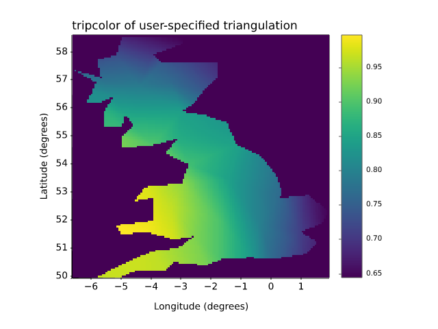
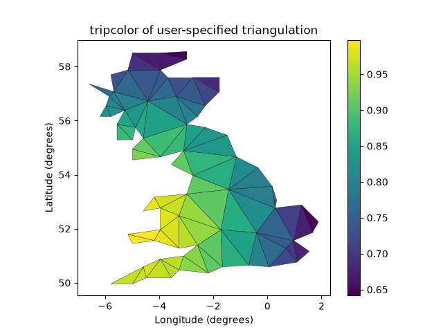
images_contours_and_fields/triplot_demo
============
Source
"""
============
Triplot Demo
============

Creating and plotting unstructured triangular grids.
"""
import matplotlib.pyplot as plt
import numpy as np

import matplotlib.tri as tri

# %%
# Creating a Triangulation without specifying the triangles results in the
# Delaunay triangulation of the points.

# First create the x and y coordinates of the points.
n_angles = 36
n_radii = 8
min_radius = 0.25
radii = np.linspace(min_radius, 0.95, n_radii)

angles = np.linspace(0, 2 * np.pi, n_angles, endpoint=False)
angles = np.repeat(angles[..., np.newaxis], n_radii, axis=1)
angles[:, 1::2] += np.pi / n_angles

x = (radii * np.cos(angles)).flatten()
y = (radii * np.sin(angles)).flatten()

# Create the Triangulation; no triangles so Delaunay triangulation created.
triang = tri.Triangulation(x, y)

# Mask off unwanted triangles.
triang.set_mask(np.hypot(x[triang.triangles].mean(axis=1),
                         y[triang.triangles].mean(axis=1))
                < min_radius)

# %%
# Plot the triangulation.

fig1, ax1 = plt.subplots()
ax1.set_aspect('equal')
ax1.triplot(triang, 'bo-', lw=1)
ax1.set_title('triplot of Delaunay triangulation')


# %%
# You can specify your own triangulation rather than perform a Delaunay
# triangulation of the points, where each triangle is given by the indices of
# the three points that make up the triangle, ordered in either a clockwise or
# anticlockwise manner.

xy = np.asarray([
    [-0.101, 0.872], [-0.080, 0.883], [-0.069, 0.888], [-0.054, 0.890],
    [-0.045, 0.897], [-0.057, 0.895], [-0.073, 0.900], [-0.087, 0.898],
    [-0.090, 0.904], [-0.069, 0.907], [-0.069, 0.921], [-0.080, 0.919],
    [-0.073, 0.928], [-0.052, 0.930], [-0.048, 0.942], [-0.062, 0.949],
    [-0.054, 0.958], [-0.069, 0.954], [-0.087, 0.952], [-0.087, 0.959],
    [-0.080, 0.966], [-0.085, 0.973], [-0.087, 0.965], [-0.097, 0.965],
    [-0.097, 0.975], [-0.092, 0.984], [-0.101, 0.980], [-0.108, 0.980],
    [-0.104, 0.987], [-0.102, 0.993], [-0.115, 1.001], [-0.099, 0.996],
    [-0.101, 1.007], [-0.090, 1.010], [-0.087, 1.021], [-0.069, 1.021],
    [-0.052, 1.022], [-0.052, 1.017], [-0.069, 1.010], [-0.064, 1.005],
    [-0.048, 1.005], [-0.031, 1.005], [-0.031, 0.996], [-0.040, 0.987],
    [-0.045, 0.980], [-0.052, 0.975], [-0.040, 0.973], [-0.026, 0.968],
    [-0.020, 0.954], [-0.006, 0.947], [ 0.003, 0.935], [ 0.006, 0.926],
    [ 0.005, 0.921], [ 0.022, 0.923], [ 0.033, 0.912], [ 0.029, 0.905],
    [ 0.017, 0.900], [ 0.012, 0.895], [ 0.027, 0.893], [ 0.019, 0.886],
    [ 0.001, 0.883], [-0.012, 0.884], [-0.029, 0.883], [-0.038, 0.879],
    [-0.057, 0.881], [-0.062, 0.876], [-0.078, 0.876], [-0.087, 0.872],
    [-0.030, 0.907], [-0.007, 0.905], [-0.057, 0.916], [-0.025, 0.933],
    [-0.077, 0.990], [-0.059, 0.993]])
x = np.degrees(xy[:, 0])
y = np.degrees(xy[:, 1])

triangles = np.asarray([
    [67, 66,  1], [65,  2, 66], [ 1, 66,  2], [64,  2, 65], [63,  3, 64],
    [60, 59, 57], [ 2, 64,  3], [ 3, 63,  4], [ 0, 67,  1], [62,  4, 63],
    [57, 59, 56], [59, 58, 56], [61, 60, 69], [57, 69, 60], [ 4, 62, 68],
    [ 6,  5,  9], [61, 68, 62], [69, 68, 61], [ 9,  5, 70], [ 6,  8,  7],
    [ 4, 70,  5], [ 8,  6,  9], [56, 69, 57], [69, 56, 52], [70, 10,  9],
    [54, 53, 55], [56, 55, 53], [68, 70,  4], [52, 56, 53], [11, 10, 12],
    [69, 71, 68], [68, 13, 70], [10, 70, 13], [51, 50, 52], [13, 68, 71],
    [52, 71, 69], [12, 10, 13], [71, 52, 50], [71, 14, 13], [50, 49, 71],
    [49, 48, 71], [14, 16, 15], [14, 71, 48], [17, 19, 18], [17, 20, 19],
    [48, 16, 14], [48, 47, 16], [47, 46, 16], [16, 46, 45], [23, 22, 24],
    [21, 24, 22], [17, 16, 45], [20, 17, 45], [21, 25, 24], [27, 26, 28],
    [20, 72, 21], [25, 21, 72], [45, 72, 20], [25, 28, 26], [44, 73, 45],
    [72, 45, 73], [28, 25, 29], [29, 25, 31], [43, 73, 44], [73, 43, 40],
    [72, 73, 39], [72, 31, 25], [42, 40, 43], [31, 30, 29], [39, 73, 40],
    [42, 41, 40], [72, 33, 31], [32, 31, 33], [39, 38, 72], [33, 72, 38],
    [33, 38, 34], [37, 35, 38], [34, 38, 35], [35, 37, 36]])

# %%
# Rather than create a Triangulation object, can simply pass x, y and triangles
# arrays to triplot directly.  It would be better to use a Triangulation object
# if the same triangulation was to be used more than once to save duplicated
# calculations.

fig2, ax2 = plt.subplots()
ax2.set_aspect('equal')
ax2.triplot(x, y, triangles, 'go-', lw=1.0)
ax2.set_title('triplot of user-specified triangulation')
ax2.set_xlabel('Longitude (degrees)')
ax2.set_ylabel('Latitude (degrees)')

plt.show()

# %%
#
# .. admonition:: References
#
#    The use of the following functions, methods, classes and modules is shown
#    in this example:
#
#    - `matplotlib.axes.Axes.triplot` / `matplotlib.pyplot.triplot`
#    - `matplotlib.tri`
#    - `matplotlib.tri.Triangulation`
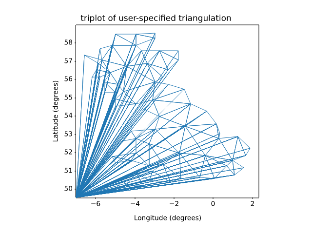
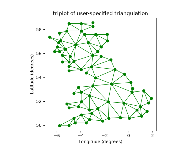
images_contours_and_fields/watermark_image
===============
Source
"""
===============
Watermark image
===============

Overlay an image on a plot by moving it to the front (``zorder=3``) and making it
semi-transparent (``alpha=0.7``).
"""

import matplotlib.pyplot as plt
import numpy as np

import matplotlib.cbook as cbook
import matplotlib.image as image

with cbook.get_sample_data('logo2.png') as file:
    im = image.imread(file)

fig, ax = plt.subplots()

np.random.seed(19680801)
x = np.arange(30)
y = x + np.random.randn(30)
ax.bar(x, y, color='#6bbc6b')
ax.grid()

fig.figimage(im, 25, 25, zorder=3, alpha=.7)

plt.show()

# %%
#
# .. admonition:: References
#
#    The use of the following functions, methods, classes and modules is shown
#    in this example:
#
#    - `matplotlib.image`
#    - `matplotlib.image.imread` / `matplotlib.pyplot.imread`
#    - `matplotlib.figure.Figure.figimage`
lines_bars_and_markers/axline
==============
Source
"""
==============
Infinite lines
==============

`~.axes.Axes.axvline` and `~.axes.Axes.axhline` draw infinite vertical /
horizontal lines, at given *x* / *y* positions. They are usually used to mark
special data values, e.g. in this example the center and limit values of the
sigmoid function.

`~.axes.Axes.axline` draws infinite straight lines defined either by two
points or by a point and a slope.

.. redirect-from:: /gallery/pyplot/axline
"""

import matplotlib.pyplot as plt
import numpy as np

t = np.linspace(-10, 10, 100)
sig = 1 / (1 + np.exp(-t))

fig, ax = plt.subplots()
ax.axhline(y=0, color="black", linestyle="--")
ax.axhline(y=0.5, color="black", linestyle=":")
ax.axhline(y=1.0, color="black", linestyle="--")
ax.axvline(color="grey")
ax.axline((0, 0.5), slope=0.25, color="black", linestyle=(0, (5, 5)))
ax.plot(t, sig, linewidth=2, label=r"$\sigma(t) = \frac{1}{1 + e^{-t}}$")
ax.set(xlim=(-10, 10), xlabel="t")
ax.legend(fontsize=14)
plt.show()

# %%
# `~.axes.Axes.axline` can also be used with a *transform* parameter, which
# applies to the point, but not to the slope. This can be useful for drawing
# diagonal grid lines with a fixed slope, which stay in place when the
# plot limits are moved.

fig, ax = plt.subplots()
for pos in np.linspace(-2, 1, 10):
    ax.axline((pos, 0), slope=0.5, color='k', transform=ax.transAxes)

ax.set(xlim=(0, 1), ylim=(0, 1))
plt.show()

# %%
#
# .. admonition:: References
#
#    The use of the following functions, methods, classes and modules is shown
#    in this example:
#
#    - `matplotlib.axes.Axes.axhline` / `matplotlib.pyplot.axhline`
#    - `matplotlib.axes.Axes.axvline` / `matplotlib.pyplot.axvline`
#    - `matplotlib.axes.Axes.axline` / `matplotlib.pyplot.axline`
#
#
# .. seealso::
#
#    `~.Axes.axhspan`, `~.Axes.axvspan` draw rectangles that span the Axes in one
#    direction and are bounded in the other direction.
#
# .. tags:: component: annotation
lines_bars_and_markers/bar_colors
====================================
Source
"""
====================================
Bar chart with individual bar colors
====================================

This is an example showing how to control bar color and legend entries
using the *color* and *label* parameters of `~matplotlib.pyplot.bar`.
Note that labels with a preceding underscore won't show up in the legend.
"""

import matplotlib.pyplot as plt

fig, ax = plt.subplots()

fruits = ['apple', 'blueberry', 'cherry', 'orange']
counts = [40, 100, 30, 55]
bar_labels = ['red', 'blue', '_red', 'orange']
bar_colors = ['tab:red', 'tab:blue', 'tab:red', 'tab:orange']

ax.bar(fruits, counts, label=bar_labels, color=bar_colors)

ax.set_ylabel('fruit supply')
ax.set_title('Fruit supply by kind and color')
ax.legend(title='Fruit color')

plt.show()

# %%
# .. tags::
#
#    styling: color
#    plot-type: bar
#    level: beginner
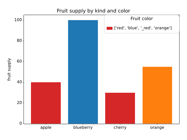
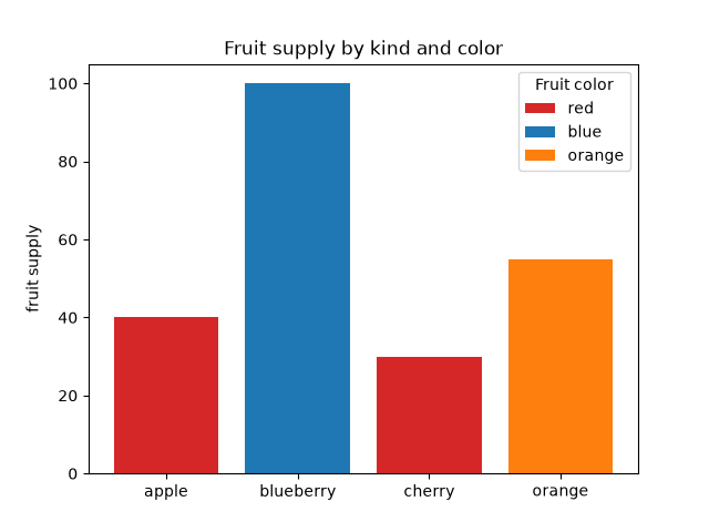
lines_bars_and_markers/bar_label_demo
=====================
Source
"""
=====================
Bar chart with labels
=====================

This example shows how to use the `~.Axes.bar_label` helper function
to create bar chart labels.

See also the :doc:`grouped bar
</gallery/lines_bars_and_markers/barchart>`,
:doc:`stacked bar
</gallery/lines_bars_and_markers/bar_stacked>` and
:doc:`horizontal bar chart
</gallery/lines_bars_and_markers/barh>` examples.
"""

import matplotlib.pyplot as plt
import numpy as np

# %%
# data from https://allisonhorst.github.io/palmerpenguins/

species = ('Adelie', 'Chinstrap', 'Gentoo')
sex_counts = {
    'Male': np.array([73, 34, 61]),
    'Female': np.array([73, 34, 58]),
}
width = 0.6  # the width of the bars: can also be len(x) sequence


fig, ax = plt.subplots()
bottom = np.zeros(3)

for sex, sex_count in sex_counts.items():
    p = ax.bar(species, sex_count, width, label=sex, bottom=bottom)
    bottom += sex_count

    ax.bar_label(p, label_type='center')

ax.set_title('Number of penguins by sex')
ax.legend()

plt.show()

# %%
# Horizontal bar chart

# Fixing random state for reproducibility
np.random.seed(19680801)

# Example data
people = ('Tom', 'Dick', 'Harry', 'Slim', 'Jim')
y_pos = np.arange(len(people))
performance = 3 + 10 * np.random.rand(len(people))
error = np.random.rand(len(people))

fig, ax = plt.subplots()

hbars = ax.barh(y_pos, performance, xerr=error, align='center')
ax.set_yticks(y_pos, labels=people)
ax.invert_yaxis()  # labels read top-to-bottom
ax.set_xlabel('Performance')
ax.set_title('How fast do you want to go today?')

# Label with specially formatted floats
ax.bar_label(hbars, fmt='%.2f')
ax.set_xlim(right=15)  # adjust xlim to fit labels

plt.show()

# %%
# Some of the more advanced things that one can do with bar labels

fig, ax = plt.subplots()

hbars = ax.barh(y_pos, performance, xerr=error, align='center')
ax.set_yticks(y_pos, labels=people)
ax.invert_yaxis()  # labels read top-to-bottom
ax.set_xlabel('Performance')
ax.set_title('How fast do you want to go today?')

# Label with given captions, custom padding and annotate options
ax.bar_label(hbars, labels=[f'±{e:.2f}' for e in error],
             padding=8, color='b', fontsize=14)
ax.set_xlim(right=16)

plt.show()

# %%
# Bar labels using {}-style format string

fruit_names = ['Coffee', 'Salted Caramel', 'Pistachio']
fruit_counts = [4000, 2000, 7000]

fig, ax = plt.subplots()
bar_container = ax.bar(fruit_names, fruit_counts)
ax.set(ylabel='pints sold', title='Gelato sales by flavor', ylim=(0, 8000))
ax.bar_label(bar_container, fmt='{:,.0f}')

# %%
# Bar labels using a callable

animal_names = ['Lion', 'Gazelle', 'Cheetah']
mph_speed = [50, 60, 75]

fig, ax = plt.subplots()
bar_container = ax.bar(animal_names, mph_speed)
ax.set(ylabel='speed in MPH', title='Running speeds', ylim=(0, 80))
ax.bar_label(bar_container, fmt=lambda x: f'{x * 1.61:.1f} km/h')

# %%
#
# .. admonition:: References
#
#    The use of the following functions, methods, classes and modules is shown
#    in this example:
#
#    - `matplotlib.axes.Axes.bar` / `matplotlib.pyplot.bar`
#    - `matplotlib.axes.Axes.barh` / `matplotlib.pyplot.barh`
#    - `matplotlib.axes.Axes.bar_label` / `matplotlib.pyplot.bar_label`
#
# .. tags::
#
#    component: label
#    plot-type: bar
#    level: beginner
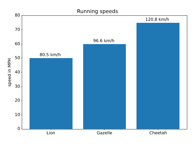
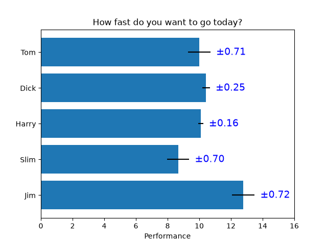
lines_bars_and_markers/bar_stacked
=================
Source
"""
=================
Stacked bar chart
=================

This is an example of creating a stacked bar plot
using `~matplotlib.pyplot.bar`.
"""

import matplotlib.pyplot as plt
import numpy as np

# data from https://allisonhorst.github.io/palmerpenguins/

species = (
    "Adelie\n $\\mu=$3700.66g",
    "Chinstrap\n $\\mu=$3733.09g",
    "Gentoo\n $\\mu=5076.02g$",
)
weight_counts = {
    "Below": np.array([70, 31, 58]),
    "Above": np.array([82, 37, 66]),
}
width = 0.5

fig, ax = plt.subplots()
bottom = np.zeros(3)

for boolean, weight_count in weight_counts.items():
    p = ax.bar(species, weight_count, width, label=boolean, bottom=bottom)
    bottom += weight_count

ax.set_title("Number of penguins with above average body mass")
ax.legend(loc="upper right")

plt.show()

# %%
# .. tags::
#
#    plot-type: bar
#    level: beginner
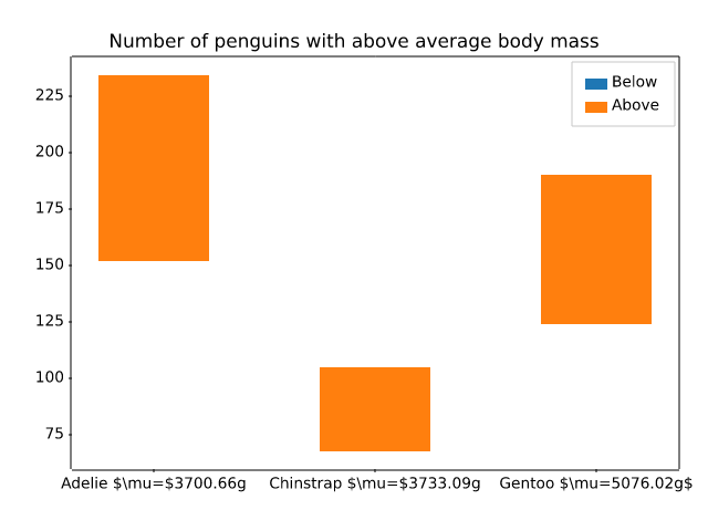
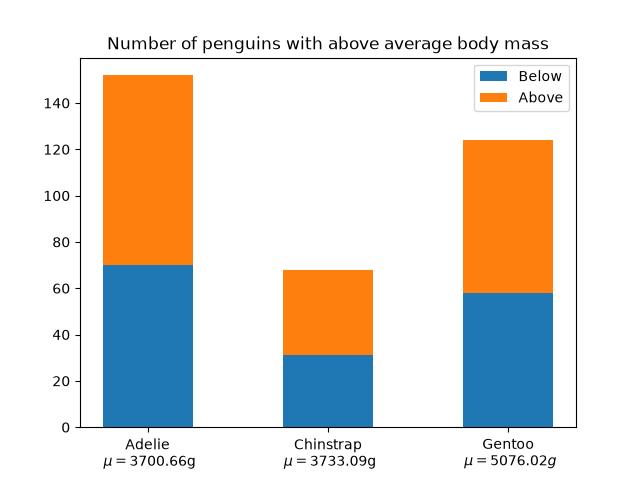
lines_bars_and_markers/barchart
=============================
Source
"""
=============================
Grouped bar chart with labels
=============================

This example shows a how to create a grouped bar chart and how to annotate
bars with labels.
"""

# data from https://allisonhorst.github.io/palmerpenguins/

import matplotlib.pyplot as plt

species = ("Adelie", "Chinstrap", "Gentoo")
penguin_means = {
    'Bill Depth': (18.35, 18.43, 14.98),
    'Bill Length': (38.79, 48.83, 47.50),
    'Flipper Length': (189.95, 195.82, 217.19),
}

fig, ax = plt.subplots(layout='constrained')

res = ax.grouped_bar(penguin_means, tick_labels=species, group_spacing=1)
for container in res.bar_containers:
    ax.bar_label(container, padding=3)

# Add some text for labels, title, etc.
ax.set_ylabel('Length (mm)')
ax.set_title('Penguin attributes by species')
ax.legend(loc='upper left', ncols=3)
ax.set_ylim(0, 250)

plt.show()

# %%
#
# .. admonition:: References
#
#    The use of the following functions, methods, classes and modules is shown
#    in this example:
#
#    - `matplotlib.axes.Axes.bar` / `matplotlib.pyplot.bar`
#    - `matplotlib.axes.Axes.bar_label` / `matplotlib.pyplot.bar_label`
#
# .. tags::
#
#    component: label
#    plot-type: bar
#    level: beginner
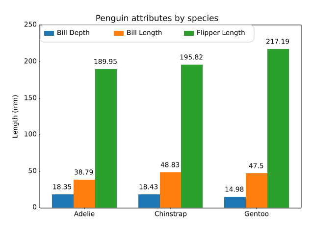
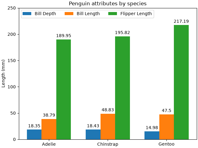
lines_bars_and_markers/barh
====================
Source
"""
====================
Horizontal bar chart
====================

This example showcases a simple horizontal bar chart.
"""
import matplotlib.pyplot as plt

fig, ax = plt.subplots()

# Example data
people = ('Tom', 'Dick', 'Harry', 'Slim', 'Jim')
performance = [5, 7, 6, 4, 9]
error = [0.2, 0.4, 0.3, 0.6, 0.2]

ax.barh(people, performance, xerr=error, align='center')
ax.yaxis.set_inverted(True)  # arrange data from top to bottom
ax.set_xlabel('Performance')
ax.set_title('How fast do you want to go today?')

plt.show()

# %%
# .. tags::
#
#    plot-type: bar
#    level: beginner
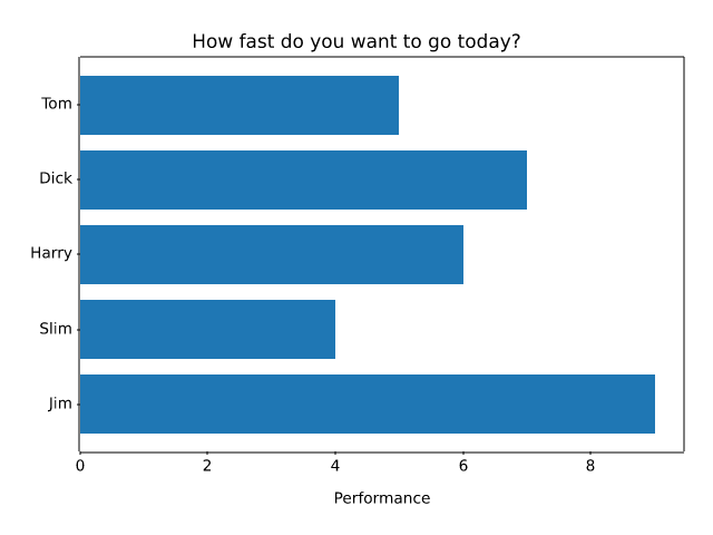
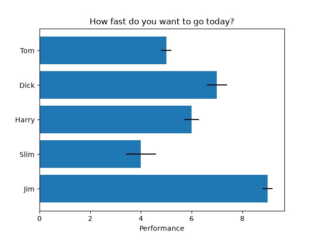
lines_bars_and_markers/broken_barh
======================
Source
"""
======================
Broken horizontal bars
======================

`~.Axes.broken_barh` creates sequences of horizontal bars. This example shows
a timing diagram.
"""
import matplotlib.pyplot as plt
import numpy as np

# data is a sequence of (start, duration) tuples
cpu_1 = [(0, 3), (3.5, 1), (5, 5)]
cpu_2 = np.column_stack([np.linspace(0, 9, 10), np.full(10, 0.5)])
cpu_3 = np.column_stack([10*np.random.random(61), np.full(61, 0.05)])
cpu_4 = [(2, 1.7), (7, 1.2)]
disk = [(1, 1.5)]
network = np.column_stack([10*np.random.random(10), np.full(10, 0.05)])

fig, ax = plt.subplots()
# broken_barh(xranges, (ypos, height))
ax.broken_barh(cpu_1, ("CPU 1", 0.4), align="center")
ax.broken_barh(cpu_2, ("CPU 2", 0.4), align="center")
ax.broken_barh(cpu_3, ("CPU 3", 0.4), align="center")
ax.broken_barh(cpu_4, ("CPU 4", 0.4), align="center")
ax.broken_barh(disk, ("disk", 0.4), align="center", color="tab:orange")
ax.broken_barh(network, ("network", 0.4), align="center", color="tab:green")
ax.set_xlim(0, 10)
ax.invert_yaxis()  # order the bars from top to bottom
ax.set_title("Resource usage")

plt.show()
# %%
#
# .. admonition:: References
#
#    The use of the following functions, methods, classes and modules is shown
#    in this example:
#
#    - `matplotlib.axes.Axes.broken_barh` / `matplotlib.pyplot.broken_barh`
#    - `matplotlib.axes.Axes.invert_yaxis`
#    - `matplotlib.axes.Axes.set_yticks`
#
# .. tags::
#
#    component: annotation
#    plot-type: bar
#    level: beginner
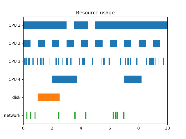
lines_bars_and_markers/capstyle
=========
Source
"""
=========
CapStyle
=========

The `matplotlib._enums.CapStyle` controls how Matplotlib draws the two
endpoints (caps) of an unclosed line. For more details, see the
`~matplotlib._enums.CapStyle` docs.
"""

import matplotlib.pyplot as plt

from matplotlib._enums import CapStyle

CapStyle.demo()
plt.show()

# %%
# .. tags::
#
#    purpose: reference

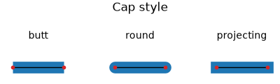
lines_bars_and_markers/categorical_variables
==============================
Source
"""
==============================
Plotting categorical variables
==============================

You can pass categorical values (i.e. strings) directly as x- or y-values to
many plotting functions:
"""
import matplotlib.pyplot as plt

data = {'apple': 10, 'orange': 15, 'lemon': 5, 'lime': 20}
names = list(data.keys())
values = list(data.values())

fig, axs = plt.subplots(1, 3, figsize=(9, 3), sharey=True)
axs[0].bar(names, values)
axs[1].scatter(names, values)
axs[2].plot(names, values)
fig.suptitle('Categorical Plotting')


# %%
# Categorical values are a mapping from names to positions. This means that
# values that occur multiple times are mapped to the same position. See the
# ``cat`` and ``dog`` values "happy" and "bored" on the y-axis in the following
# example.

cat = ["bored", "happy", "bored", "bored", "happy", "bored"]
dog = ["happy", "happy", "happy", "happy", "bored", "bored"]
activity = ["combing", "drinking", "feeding", "napping", "playing", "washing"]

fig, ax = plt.subplots()
ax.plot(activity, dog, label="dog")
ax.plot(activity, cat, label="cat")
ax.legend()

plt.show()

# %%
# .. tags::
#
#    plot-type: specialty
#    level: beginner
lines_bars_and_markers/eventcollection_demo
====================
Source
r"""
====================
EventCollection Demo
====================

Plot two curves, then use `.EventCollection`\s to mark the locations of the x
and y data points on the respective Axes for each curve.
"""

import matplotlib.pyplot as plt
import numpy as np

from matplotlib.collections import EventCollection

# Fixing random state for reproducibility
np.random.seed(19680801)

# create random data
xdata = np.random.random([2, 10])

# split the data into two parts
xdata1 = xdata[0, :]
xdata2 = xdata[1, :]

# sort the data so it makes clean curves
xdata1.sort()
xdata2.sort()

# create some y data points
ydata1 = xdata1 ** 2
ydata2 = 1 - xdata2 ** 3

# plot the data
fig = plt.figure()
ax = fig.add_subplot(1, 1, 1)
ax.plot(xdata1, ydata1, color='tab:blue')
ax.plot(xdata2, ydata2, color='tab:orange')

# create the events marking the x data points
xevents1 = EventCollection(xdata1, color='tab:blue', linelength=0.05)
xevents2 = EventCollection(xdata2, color='tab:orange', linelength=0.05)

# create the events marking the y data points
yevents1 = EventCollection(ydata1, color='tab:blue', linelength=0.05,
                           orientation='vertical')
yevents2 = EventCollection(ydata2, color='tab:orange', linelength=0.05,
                           orientation='vertical')

# add the events to the axis
ax.add_collection(xevents1)
ax.add_collection(xevents2)
ax.add_collection(yevents1)
ax.add_collection(yevents2)

# set the limits
ax.set_xlim(0, 1)
ax.set_ylim(0, 1)

ax.set_title('line plot with data points')

# display the plot
plt.show()

# %%
# .. tags::
#
#    plot-type: eventplot
#    level: intermediate
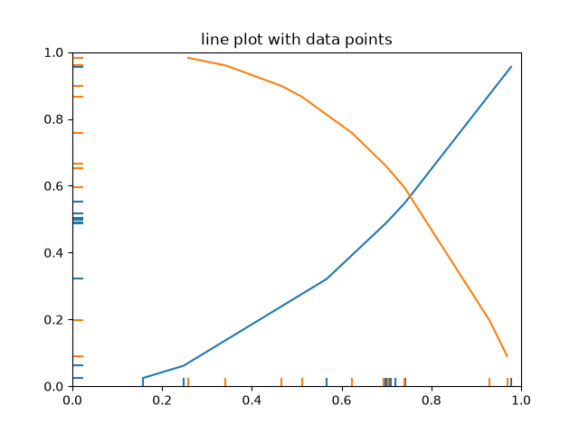
lines_bars_and_markers/eventplot_demo
==============
Source
"""
==============
Eventplot demo
==============

An `~.axes.Axes.eventplot` showing sequences of events with various line
properties. The plot is shown in both horizontal and vertical orientations.
"""

import matplotlib.pyplot as plt
import numpy as np

import matplotlib

matplotlib.rcParams['font.size'] = 8.0

# Fixing random state for reproducibility
np.random.seed(19680801)


# create random data
data1 = np.random.random([6, 50])

# set different colors for each set of positions
colors1 = [f'C{i}' for i in range(6)]

# set different line properties for each set of positions
# note that some overlap
lineoffsets1 = [-15, -3, 1, 1.5, 6, 10]
linelengths1 = [5, 2, 1, 1, 3, 1.5]

fig, axs = plt.subplots(2, 2)

# create a horizontal plot
axs[0, 0].eventplot(data1, colors=colors1, lineoffsets=lineoffsets1,
                    linelengths=linelengths1)

# create a vertical plot
axs[1, 0].eventplot(data1, colors=colors1, lineoffsets=lineoffsets1,
                    linelengths=linelengths1, orientation='vertical')

# create another set of random data.
# the gamma distribution is only used for aesthetic purposes
data2 = np.random.gamma(4, size=[60, 50])

# use individual values for the parameters this time
# these values will be used for all data sets (except lineoffsets2, which
# sets the increment between each data set in this usage)
colors2 = 'black'
lineoffsets2 = 1
linelengths2 = 1

# create a horizontal plot
axs[0, 1].eventplot(data2, colors=colors2, lineoffsets=lineoffsets2,
                    linelengths=linelengths2)


# create a vertical plot
axs[1, 1].eventplot(data2, colors=colors2, lineoffsets=lineoffsets2,
                    linelengths=linelengths2, orientation='vertical')

plt.show()

# %%
# .. tags::
#
#    plot-type: eventplot
#    level: beginner
#    purpose: showcase
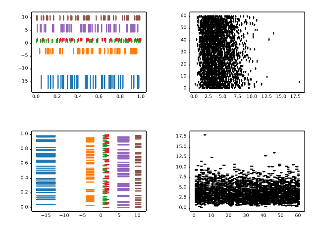
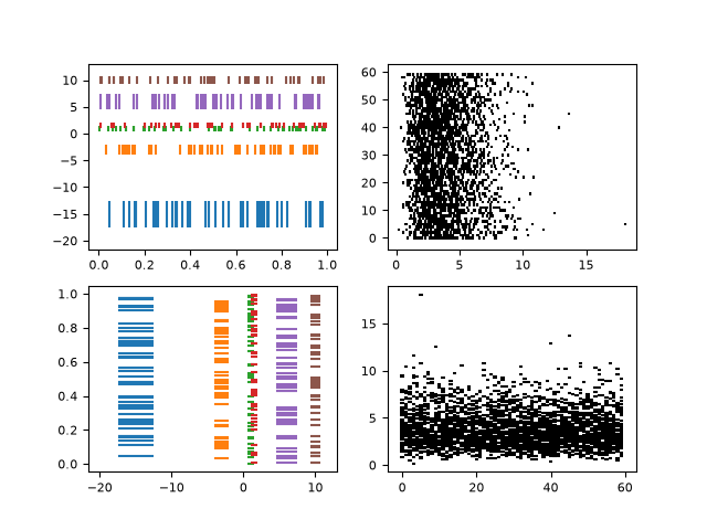
lines_bars_and_markers/fill
==============
Source
"""
==============
Filled polygon
==============

`~.Axes.fill()` draws a filled polygon based on lists of point
coordinates *x*, *y*.

This example uses the `Koch snowflake`_ as an example polygon.

.. _Koch snowflake: https://en.wikipedia.org/wiki/Koch_snowflake

"""

import matplotlib.pyplot as plt
import numpy as np


def koch_snowflake(order, scale=10):
    """
    Return two lists x, y of point coordinates of the Koch snowflake.

    Parameters
    ----------
    order : int
        The recursion depth.
    scale : float
        The extent of the snowflake (edge length of the base triangle).
    """
    def _koch_snowflake_complex(order):
        if order == 0:
            # initial triangle
            angles = np.array([0, 120, 240]) + 90
            return scale / np.sqrt(3) * np.exp(np.deg2rad(angles) * 1j)
        else:
            ZR = 0.5 - 0.5j * np.sqrt(3) / 3

            p1 = _koch_snowflake_complex(order - 1)  # start points
            p2 = np.roll(p1, shift=-1)  # end points
            dp = p2 - p1  # connection vectors

            new_points = np.empty(len(p1) * 4, dtype=np.complex128)
            new_points[::4] = p1
            new_points[1::4] = p1 + dp / 3
            new_points[2::4] = p1 + dp * ZR
            new_points[3::4] = p1 + dp / 3 * 2
            return new_points

    points = _koch_snowflake_complex(order)
    x, y = points.real, points.imag
    return x, y


# %%
# Basic usage:

x, y = koch_snowflake(order=5)

plt.figure(figsize=(8, 8))
plt.axis('equal')
plt.fill(x, y)
plt.show()

# %%
# Use keyword arguments *facecolor* and *edgecolor* to modify the colors
# of the polygon. Since the *linewidth* of the edge is 0 in the default
# Matplotlib style, we have to set it as well for the edge to become visible.

x, y = koch_snowflake(order=2)

fig, (ax1, ax2, ax3) = plt.subplots(1, 3, figsize=(9, 3),
                                    subplot_kw={'aspect': 'equal'})
ax1.fill(x, y)
ax2.fill(x, y, facecolor='lightsalmon', edgecolor='orangered', linewidth=3)
ax3.fill(x, y, facecolor='none', edgecolor='purple', linewidth=3)

plt.show()

# %%
#
# .. admonition:: References
#
#    The use of the following functions, methods, classes and modules is shown
#    in this example:
#
#    - `matplotlib.axes.Axes.fill` / `matplotlib.pyplot.fill`
#    - `matplotlib.axes.Axes.axis` / `matplotlib.pyplot.axis`
#
# .. tags::
#
#    styling: shape
#    level: beginner
#    purpose: showcase
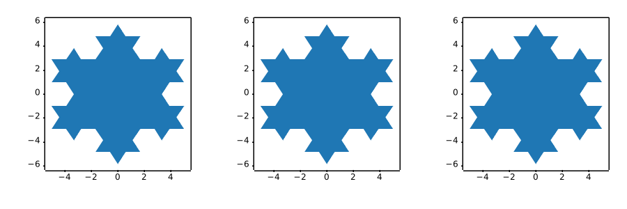
lines_bars_and_markers/fill_between_alpha
==================================
Source
"""
==================================
``fill_between`` with transparency
==================================

The `~matplotlib.axes.Axes.fill_between` function generates a shaded
region between a min and max boundary that is useful for illustrating ranges.
It has a very handy ``where`` argument to combine filling with logical ranges,
e.g., to just fill in a curve over some threshold value.

At its most basic level, ``fill_between`` can be used to enhance a graph's
visual appearance. Let's compare two graphs of financial data with a simple
line plot on the left and a filled line on the right.
"""

import matplotlib.pyplot as plt
import numpy as np

import matplotlib.cbook as cbook

# load up some sample financial data
r = cbook.get_sample_data('goog.npz')['price_data']
# create two subplots with the shared x and y axes
fig, (ax1, ax2) = plt.subplots(1, 2, sharex=True, sharey=True)

pricemin = r["close"].min()

ax1.plot(r["date"], r["close"], lw=2)
ax2.fill_between(r["date"], pricemin, r["close"], alpha=0.7)

for ax in ax1, ax2:
    ax.grid(True)
    ax.label_outer()

ax1.set_ylabel('price')

fig.suptitle('Google (GOOG) daily closing price')
fig.autofmt_xdate()

# %%
# The alpha channel is not necessary here, but it can be used to soften
# colors for more visually appealing plots.  In other examples, as we'll
# see below, the alpha channel is functionally useful as the shaded
# regions can overlap and alpha allows you to see both.  Note that the
# postscript format does not support alpha (this is a postscript
# limitation, not a matplotlib limitation), so when using alpha save
# your figures in GIF, PNG, PDF or SVG.
#
# Our next example computes two populations of random walkers with a
# different mean and standard deviation of the normal distributions from
# which the steps are drawn.  We use filled regions to plot +/- one
# standard deviation of the mean position of the population.  Here the
# alpha channel is useful, not just aesthetic.

# Fixing random state for reproducibility
np.random.seed(19680801)

Nsteps, Nwalkers = 100, 250
t = np.arange(Nsteps)

# an (Nsteps x Nwalkers) array of random walk steps
S1 = 0.004 + 0.02*np.random.randn(Nsteps, Nwalkers)
S2 = 0.002 + 0.01*np.random.randn(Nsteps, Nwalkers)

# an (Nsteps x Nwalkers) array of random walker positions
X1 = S1.cumsum(axis=0)
X2 = S2.cumsum(axis=0)


# Nsteps length arrays empirical means and standard deviations of both
# populations over time
mu1 = X1.mean(axis=1)
sigma1 = X1.std(axis=1)
mu2 = X2.mean(axis=1)
sigma2 = X2.std(axis=1)

# plot it!
fig, ax = plt.subplots(1)
ax.plot(t, mu1, lw=2, label='mean population 1')
ax.plot(t, mu2, lw=2, label='mean population 2')
ax.fill_between(t, mu1+sigma1, mu1-sigma1, facecolor='C0', alpha=0.4)
ax.fill_between(t, mu2+sigma2, mu2-sigma2, facecolor='C1', alpha=0.4)
ax.set_title(r'random walkers empirical $\mu$ and $\pm \sigma$ interval')
ax.legend(loc='upper left')
ax.set_xlabel('num steps')
ax.set_ylabel('position')
ax.grid()

# %%
# The ``where`` keyword argument is very handy for highlighting certain
# regions of the graph.  ``where`` takes a boolean mask the same length
# as the x, ymin and ymax arguments, and only fills in the region where
# the boolean mask is True.  In the example below, we simulate a single
# random walker and compute the analytic mean and standard deviation of
# the population positions.  The population mean is shown as the dashed
# line, and the plus/minus one sigma deviation from the mean is shown
# as the filled region.  We use the where mask ``X > upper_bound`` to
# find the region where the walker is outside the one sigma boundary,
# and shade that region red.

# Fixing random state for reproducibility
np.random.seed(1)

Nsteps = 500
t = np.arange(Nsteps)

mu = 0.002
sigma = 0.01

# the steps and position
S = mu + sigma*np.random.randn(Nsteps)
X = S.cumsum()

# the 1 sigma upper and lower analytic population bounds
lower_bound = mu*t - sigma*np.sqrt(t)
upper_bound = mu*t + sigma*np.sqrt(t)

fig, ax = plt.subplots(1)
ax.plot(t, X, lw=2, label='walker position')
ax.plot(t, mu*t, lw=1, label='population mean', color='C0', ls='--')
ax.fill_between(t, lower_bound, upper_bound, facecolor='C0', alpha=0.4,
                label='1 sigma range')
ax.legend(loc='upper left')

# here we use the where argument to only fill the region where the
# walker is above the population 1 sigma boundary
ax.fill_between(t, upper_bound, X, where=X > upper_bound, fc='red', alpha=0.4)
ax.fill_between(t, lower_bound, X, where=X < lower_bound, fc='red', alpha=0.4)
ax.set_xlabel('num steps')
ax.set_ylabel('position')
ax.grid()

# %%
# Another handy use of filled regions is to highlight horizontal or vertical
# spans of an Axes -- for that Matplotlib has the helper functions
# `~matplotlib.axes.Axes.axhspan` and `~matplotlib.axes.Axes.axvspan`.  See
# :doc:`/gallery/subplots_axes_and_figures/axhspan_demo`.

plt.show()

# %%
# .. tags::
#
#    styling: alpha
#    plot-type: fill_between
#    level: intermediate
#    purpose: showcase
lines_bars_and_markers/fill_between_demo
===============================
Source
"""
===============================
Fill the area between two lines
===============================

This example shows how to use `~.axes.Axes.fill_between` to color the area
between two lines.
"""

import matplotlib.pyplot as plt
import numpy as np

# %%
#
# Basic usage
# -----------
# The parameters *y1* and *y2* can be scalars, indicating a horizontal
# boundary at the given y-values. If only *y1* is given, *y2* defaults to 0.

x = np.arange(0.0, 2, 0.01)
y1 = np.sin(2 * np.pi * x)
y2 = 0.8 * np.sin(4 * np.pi * x)

fig, (ax1, ax2, ax3) = plt.subplots(3, 1, sharex=True, figsize=(6, 6))

ax1.fill_between(x, y1)
ax1.set_title('fill between y1 and 0')

ax2.fill_between(x, y1, 1)
ax2.set_title('fill between y1 and 1')

ax3.fill_between(x, y1, y2)
ax3.set_title('fill between y1 and y2')
ax3.set_xlabel('x')
fig.tight_layout()

# %%
#
# Example: Confidence bands
# -------------------------
# A common application for `~.axes.Axes.fill_between` is the indication of
# confidence bands.
#
# `~.axes.Axes.fill_between` uses the colors of the color cycle as the fill
# color. These may be a bit strong when applied to fill areas. It is
# therefore often a good practice to lighten the color by making the area
# semi-transparent using *alpha*.

# sphinx_gallery_thumbnail_number = 2

N = 21
x = np.linspace(0, 10, 11)
y = [3.9, 4.4, 10.8, 10.3, 11.2, 13.1, 14.1,  9.9, 13.9, 15.1, 12.5]

# fit a linear curve and estimate its y-values and their error.
a, b = np.polyfit(x, y, deg=1)
y_est = a * x + b
y_err = x.std() * np.sqrt(1/len(x) +
                          (x - x.mean())**2 / np.sum((x - x.mean())**2))

fig, ax = plt.subplots()
ax.plot(x, y_est, '-')
ax.fill_between(x, y_est - y_err, y_est + y_err, alpha=0.2)
ax.plot(x, y, 'o', color='tab:brown')

# %%
#
# Selectively filling horizontal regions
# --------------------------------------
# The parameter *where* allows to specify the x-ranges to fill. It's a boolean
# array with the same size as *x*.
#
# Only x-ranges of contiguous *True* sequences are filled. As a result the
# range between neighboring *True* and *False* values is never filled. This
# often undesired when the data points should represent a contiguous quantity.
# It is therefore recommended to set ``interpolate=True`` unless the
# x-distance of the data points is fine enough so that the above effect is not
# noticeable. Interpolation approximates the actual x position at which the
# *where* condition will change and extends the filling up to there.

x = np.array([0, 1, 2, 3])
y1 = np.array([0.8, 0.8, 0.2, 0.2])
y2 = np.array([0, 0, 1, 1])

fig, (ax1, ax2) = plt.subplots(2, 1, sharex=True)

ax1.set_title('interpolation=False')
ax1.plot(x, y1, 'o--')
ax1.plot(x, y2, 'o--')
ax1.fill_between(x, y1, y2, where=(y1 > y2), color='C0', alpha=0.3)
ax1.fill_between(x, y1, y2, where=(y1 < y2), color='C1', alpha=0.3)

ax2.set_title('interpolation=True')
ax2.plot(x, y1, 'o--')
ax2.plot(x, y2, 'o--')
ax2.fill_between(x, y1, y2, where=(y1 > y2), color='C0', alpha=0.3,
                 interpolate=True)
ax2.fill_between(x, y1, y2, where=(y1 <= y2), color='C1', alpha=0.3,
                 interpolate=True)
fig.tight_layout()

# %%
#
# .. note::
#
#    Similar gaps will occur if *y1* or *y2* are masked arrays. Since missing
#    values cannot be approximated, *interpolate* has no effect in this case.
#    The gaps around masked values can only be reduced by adding more data
#    points close to the masked values.

# %%
#
# Selectively marking horizontal regions across the whole Axes
# ------------------------------------------------------------
# The same selection mechanism can be applied to fill the full vertical height
# of the Axes. To be independent of y-limits, we add a transform that
# interprets the x-values in data coordinates and the y-values in Axes
# coordinates.
#
# The following example marks the regions in which the y-data are above a
# given threshold.

fig, ax = plt.subplots()
x = np.arange(0, 4 * np.pi, 0.01)
y = np.sin(x)
ax.plot(x, y, color='black')

threshold = 0.75
ax.axhline(threshold, color='green', lw=2, alpha=0.7)
ax.fill_between(x, 0, 1, where=y > threshold,
                color='green', alpha=0.5, transform=ax.get_xaxis_transform())

# %%
#
# .. admonition:: References
#
#    The use of the following functions, methods, classes and modules is shown
#    in this example:
#
#    - `matplotlib.axes.Axes.fill_between` / `matplotlib.pyplot.fill_between`
#    - `matplotlib.axes.Axes.get_xaxis_transform`
#
# .. tags::
#
#    styling: conditional
#    plot-type: fill_between
#    level: beginner
#    purpose: showcase
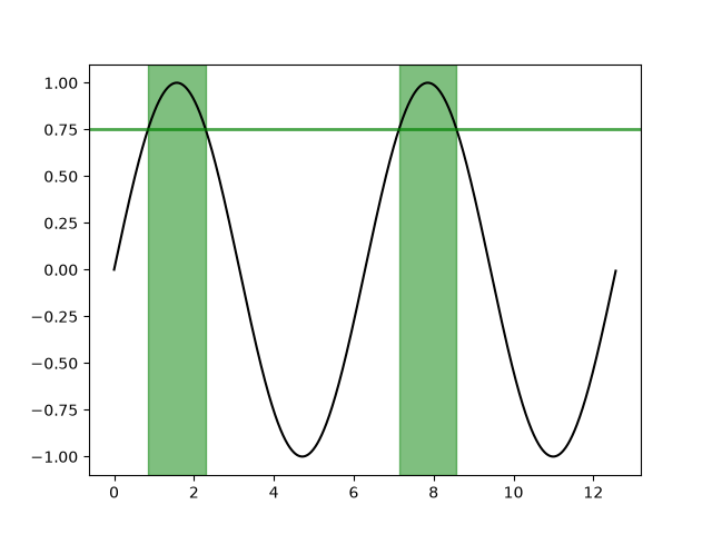
lines_bars_and_markers/fill_betweenx_demo
========================================
Source
"""
========================================
Fill the area between two vertical lines
========================================

Using `~.Axes.fill_betweenx` to color along the horizontal direction between
two curves.
"""
import matplotlib.pyplot as plt
import numpy as np

y = np.arange(0.0, 2, 0.01)
x1 = np.sin(2 * np.pi * y)
x2 = 1.2 * np.sin(4 * np.pi * y)

fig, [ax1, ax2, ax3] = plt.subplots(1, 3, sharey=True, figsize=(6, 6))

ax1.fill_betweenx(y, 0, x1)
ax1.set_title('between (x1, 0)')

ax2.fill_betweenx(y, x1, 1)
ax2.set_title('between (x1, 1)')
ax2.set_xlabel('x')

ax3.fill_betweenx(y, x1, x2)
ax3.set_title('between (x1, x2)')

# %%
# Now fill between x1 and x2 where a logical condition is met. Note this is
# different than calling::
#
#   fill_between(y[where], x1[where], x2[where])
#
# because of edge effects over multiple contiguous regions.

fig, [ax, ax1] = plt.subplots(1, 2, sharey=True, figsize=(6, 6))
ax.plot(x1, y, x2, y, color='black')
ax.fill_betweenx(y, x1, x2, where=x2 >= x1, facecolor='green')
ax.fill_betweenx(y, x1, x2, where=x2 <= x1, facecolor='red')
ax.set_title('fill_betweenx where')

# Test support for masked arrays.
x2 = np.ma.masked_greater(x2, 1.0)
ax1.plot(x1, y, x2, y, color='black')
ax1.fill_betweenx(y, x1, x2, where=x2 >= x1, facecolor='green')
ax1.fill_betweenx(y, x1, x2, where=x2 <= x1, facecolor='red')
ax1.set_title('regions with x2 > 1 are masked')

# %%
# This example illustrates a problem; because of the data gridding, there are
# undesired unfilled triangles at the crossover points. A brute-force solution
# would be to interpolate all arrays to a very fine grid before plotting.

plt.show()

# %%
# .. tags::
#
#    plot-type: fill_between
#    level: beginner
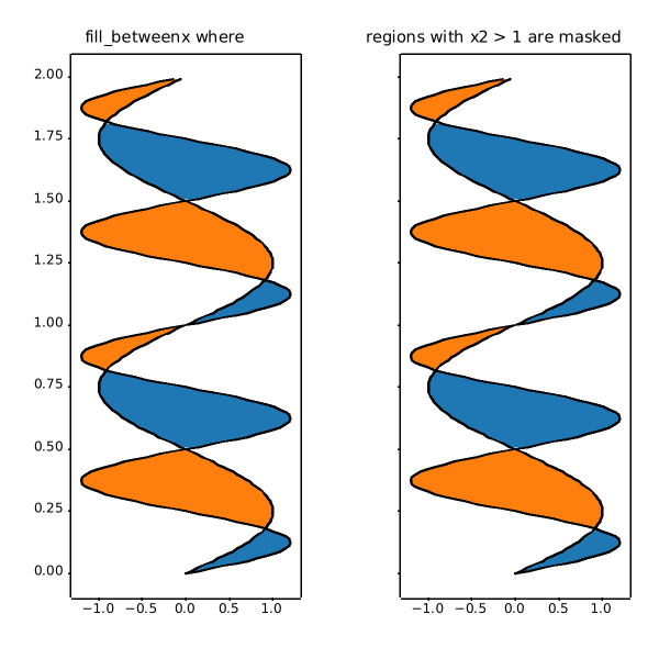
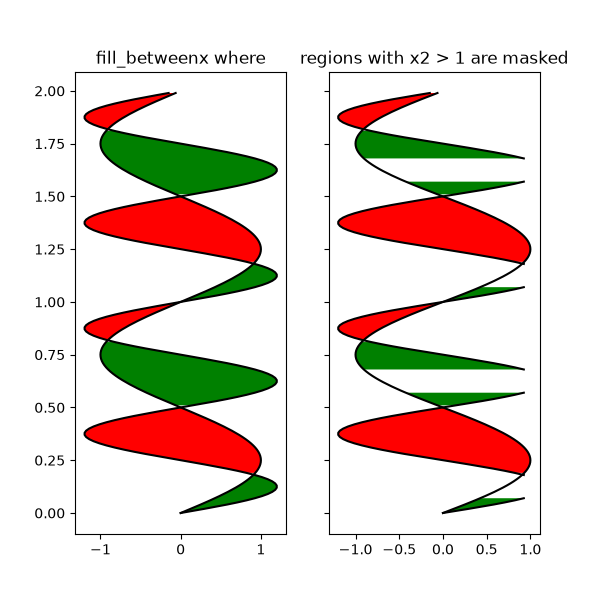
lines_bars_and_markers/gradient_bar
========================
Source
"""
========================
Bar chart with gradients
========================

Matplotlib does not natively support gradients. However, we can emulate a
gradient-filled rectangle by an `.AxesImage` of the right size and coloring.

In particular, we use a colormap to generate the actual colors. It is then
sufficient to define the underlying values on the corners of the image and
let bicubic interpolation fill out the area. We define the gradient direction
by a unit vector *v*. The values at the corners are then obtained by the
lengths of the projections of the corner vectors on *v*.

A similar approach can be used to create a gradient background for an Axes.
In that case, it is helpful to use Axes coordinates (``extent=(0, 1, 0, 1),
transform=ax.transAxes``) to be independent of the data coordinates.
"""

import matplotlib.pyplot as plt
import numpy as np

np.random.seed(19680801)


def gradient_image(ax, direction=0.3, cmap_range=(0, 1), **kwargs):
    """
    Draw a gradient image based on a colormap.

    Parameters
    ----------
    ax : Axes
        The Axes to draw on.
    direction : float
        The direction of the gradient. This is a number in
        range 0 (=vertical) to 1 (=horizontal).
    cmap_range : float, float
        The fraction (cmin, cmax) of the colormap that should be
        used for the gradient, where the complete colormap is (0, 1).
    **kwargs
        Other parameters are passed on to `.Axes.imshow()`.
        In particular, *cmap*, *extent*, and *transform* may be useful.
    """
    phi = direction * np.pi / 2
    v = np.array([np.cos(phi), np.sin(phi)])
    X = np.array([[v @ [1, 0], v @ [1, 1]],
                  [v @ [0, 0], v @ [0, 1]]])
    a, b = cmap_range
    X = a + (b - a) / X.max() * X
    im = ax.imshow(X, interpolation='bicubic', clim=(0, 1),
                   aspect='auto', **kwargs)
    return im


def gradient_bar(ax, x, y, width=0.5, bottom=0):
    for left, top in zip(x, y):
        right = left + width
        gradient_image(ax, extent=(left, right, bottom, top),
                       cmap="Blues_r", cmap_range=(0, 0.8))


fig, ax = plt.subplots()
ax.set(xlim=(0, 10), ylim=(0, 1))

# background image
gradient_image(ax, direction=1, extent=(0, 1, 0, 1), transform=ax.transAxes,
               cmap="RdYlGn", cmap_range=(0.2, 0.8), alpha=0.5)

N = 10
x = np.arange(N) + 0.15
y = np.random.rand(N)
gradient_bar(ax, x, y, width=0.7)
plt.show()

# %%
# .. tags::
#
#    styling: color
#    plot-type: imshow
#    level: intermediate
#    purpose: showcase
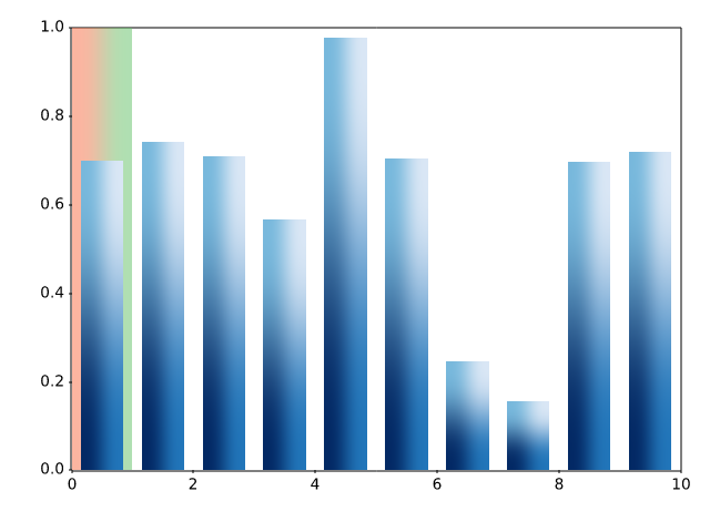
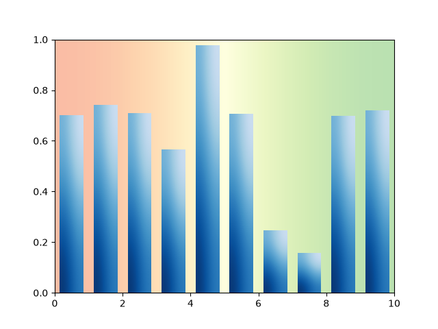
lines_bars_and_markers/hat_graph
=========
Source
"""
=========
Hat graph
=========
This example shows how to create a `hat graph`_ and how to annotate it with
labels.

.. _hat graph: https://doi.org/10.1186/s41235-019-0182-3
"""
import matplotlib.pyplot as plt
import numpy as np


def hat_graph(ax, xlabels, values, group_labels):
    """
    Create a hat graph.

    Parameters
    ----------
    ax : matplotlib.axes.Axes
        The Axes to plot into.
    xlabels : list of str
        The category names to be displayed on the x-axis.
    values : (M, N) array-like
        The data values.
        Rows are the groups (len(group_labels) == M).
        Columns are the categories (len(xlabels) == N).
    group_labels : list of str
        The group labels displayed in the legend.
    """

    values = np.asarray(values)
    color_cycle_colors = plt.rcParams['axes.prop_cycle'].by_key()['color']

    # Draw the hats
    bars = ax.grouped_bar(
        (values - values[0]).T, bottom=values[0], tick_labels=xlabels,
        labels=group_labels, edgecolor='black', group_spacing=0.8,
        colors=['none'] + color_cycle_colors)

    # Attach a text label on top of each bar
    for bc, heights in zip(bars.bar_containers, values):
        ax.bar_label(bc, heights, padding=4)


# Initialise labels and a numpy array make sure you have
# N labels of N number of values in the array
xlabels = ['I', 'II', 'III', 'IV', 'V']
playerA = np.array([5, 15, 22, 20, 25])
playerB = np.array([25, 32, 34, 30, 27])

fig, ax = plt.subplots(layout='constrained')

hat_graph(ax, xlabels, [playerA, playerB], ['Player A', 'Player B'])

# Add some text for labels, title and custom x-axis tick labels, etc.
ax.set_xlabel('Games')
ax.set_ylabel('Score')
ax.set_ylim(0, 60)
ax.set_title('Scores by number of game and players')
ax.legend()

plt.show()
# %%
#
# .. admonition:: References
#
#    The use of the following functions, methods, classes and modules is shown
#    in this example:
#
#    - `matplotlib.axes.Axes.grouped_bar` / `matplotlib.pyplot.grouped_bar`
#    - `matplotlib.axes.Axes.bar_label` / `matplotlib.pyplot.bar_label`
#
# .. tags::
#
#    component: annotation
#    plot-type: bar
#    level: beginner
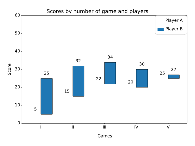
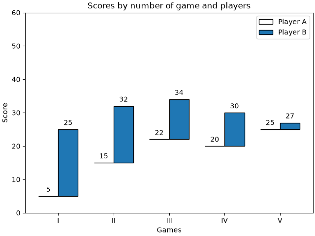
lines_bars_and_markers/horizontal_barchart_distribution
=============================================
Source
"""
=============================================
Discrete distribution as horizontal bar chart
=============================================

Stacked bar charts can be used to visualize discrete distributions.

This example visualizes the result of a survey in which people could rate
their agreement to questions on a five-element scale.

The horizontal stacking is achieved by calling `~.Axes.barh()` for each
category and passing the starting point as the cumulative sum of the
already drawn bars via the parameter ``left``.
"""

import matplotlib.pyplot as plt
import numpy as np

category_names = ['Strongly disagree', 'Disagree',
                  'Neither agree nor disagree', 'Agree', 'Strongly agree']
results = {
    'Question 1': [10, 15, 17, 32, 26],
    'Question 2': [26, 22, 29, 10, 13],
    'Question 3': [35, 37, 7, 2, 19],
    'Question 4': [32, 11, 9, 15, 33],
    'Question 5': [21, 29, 5, 5, 40],
    'Question 6': [8, 19, 5, 30, 38]
}


def survey(results, category_names):
    """
    Parameters
    ----------
    results : dict
        A mapping from question labels to a list of answers per category.
        It is assumed all lists contain the same number of entries and that
        it matches the length of *category_names*.
    category_names : list of str
        The category labels.
    """
    labels = list(results.keys())
    data = np.array(list(results.values()))
    data_cum = data.cumsum(axis=1)
    category_colors = plt.colormaps['RdYlGn'](
        np.linspace(0.15, 0.85, data.shape[1]))

    fig, ax = plt.subplots(figsize=(9.2, 5))
    ax.invert_yaxis()
    ax.xaxis.set_visible(False)
    ax.set_xlim(0, np.sum(data, axis=1).max())

    for i, (colname, color) in enumerate(zip(category_names, category_colors)):
        widths = data[:, i]
        starts = data_cum[:, i] - widths
        rects = ax.barh(labels, widths, left=starts, height=0.5,
                        label=colname, color=color)

        r, g, b, _ = color
        text_color = 'white' if r * g * b < 0.5 else 'darkgrey'
        ax.bar_label(rects, label_type='center', color=text_color)
    ax.legend(ncols=len(category_names), bbox_to_anchor=(0, 1),
              loc='lower left', fontsize='small')

    return fig, ax


survey(results, category_names)
plt.show()

# %%
#
# .. admonition:: References
#
#    The use of the following functions, methods, classes and modules is shown
#    in this example:
#
#    - `matplotlib.axes.Axes.barh` / `matplotlib.pyplot.barh`
#    - `matplotlib.axes.Axes.bar_label` / `matplotlib.pyplot.bar_label`
#    - `matplotlib.axes.Axes.legend` / `matplotlib.pyplot.legend`
#
# .. tags::
#
#    domain: statistics
#    component: label
#    plot-type: bar
#    level: beginner
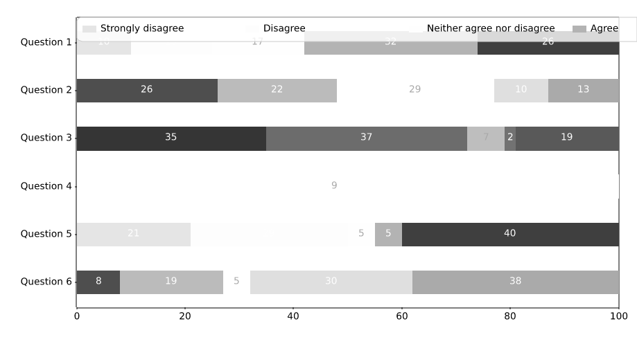
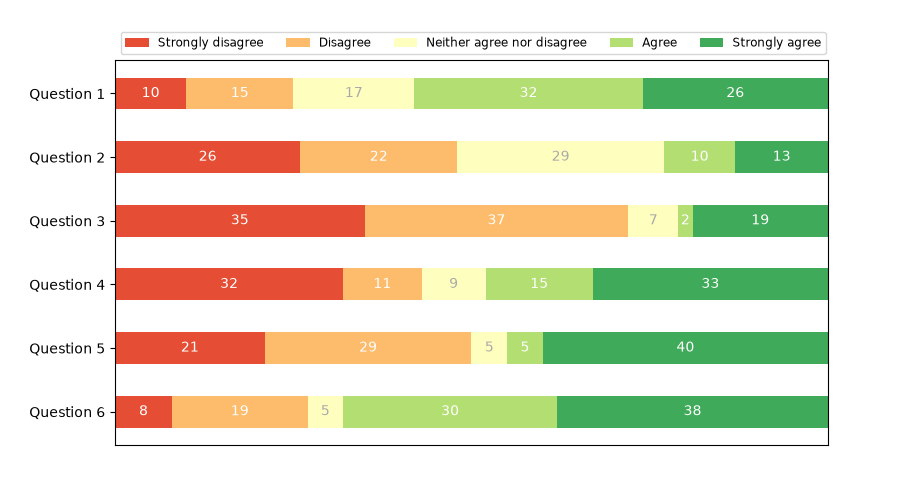
lines_bars_and_markers/joinstyle
=========
Source
"""
=========
JoinStyle
=========

The `matplotlib._enums.JoinStyle` controls how Matplotlib draws the corners
where two different line segments meet. For more details, see the
`~matplotlib._enums.JoinStyle` docs.
"""

import matplotlib.pyplot as plt

from matplotlib._enums import JoinStyle

JoinStyle.demo()
plt.show()

# %%
# .. tags:: purpose: reference, styling: linestyle

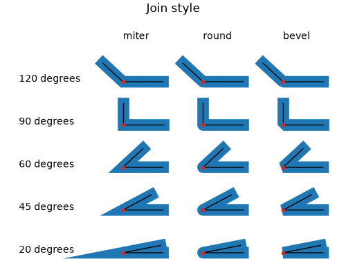
lines_bars_and_markers/line_demo_dash_control
===============================
Source
"""
===============================
Dashed line style configuration
===============================

The dashing of a line is controlled via a dash sequence. It can be modified
using `.Line2D.set_dashes`.

The dash sequence is a series of on/off lengths in points, e.g.
``[3, 1]`` would be 3pt long lines separated by 1pt spaces.

Some functions like `.Axes.plot` support passing Line properties as keyword
arguments. In such a case, you can already set the dashing when creating the
line.

*Note*: The dash style can also be configured via a
:ref:`property_cycle <color_cycle>`
by passing a list of dash sequences using the keyword *dashes* to the
cycler. This is not shown within this example.

Other attributes of the dash may also be set either with the relevant method
(`~.Line2D.set_dash_capstyle`, `~.Line2D.set_dash_joinstyle`,
`~.Line2D.set_gapcolor`) or by passing the property through a plotting
function.
"""
import matplotlib.pyplot as plt
import numpy as np

x = np.linspace(0, 10, 500)
y = np.sin(x)

plt.rc('lines', linewidth=2.5)
fig, ax = plt.subplots()

# Using set_dashes() and set_capstyle() to modify dashing of an existing line.
line1, = ax.plot(x, y, label='Using set_dashes() and set_dash_capstyle()')
line1.set_dashes([2, 2, 10, 2])  # 2pt line, 2pt break, 10pt line, 2pt break.
line1.set_dash_capstyle('round')

# Using plot(..., dashes=...) to set the dashing when creating a line.
line2, = ax.plot(x, y - 0.2, dashes=[6, 2], label='Using the dashes parameter')

# Using plot(..., dashes=..., gapcolor=...) to set the dashing and
# alternating color when creating a line.
line3, = ax.plot(x, y - 0.4, dashes=[4, 4], gapcolor='tab:pink',
                 label='Using the dashes and gapcolor parameters')

ax.legend(handlelength=4)
plt.show()

# %%
# .. tags::
#
#    styling: linestyle
#    plot-type: line
#    level: beginner
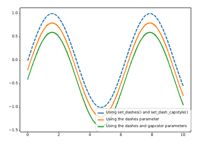
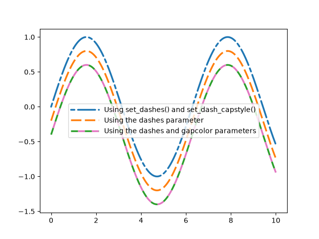
lines_bars_and_markers/lines_with_ticks_demo
==============================
Source
"""
==============================
Lines with a ticked patheffect
==============================

Ticks can be added along a line to mark one side as a barrier using
`~matplotlib.patheffects.TickedStroke`.  You can control the angle,
spacing, and length of the ticks.

The ticks will also appear appropriately in the legend.

"""

import matplotlib.pyplot as plt
import numpy as np

from matplotlib import patheffects

# Plot a straight diagonal line with ticked style path
fig, ax = plt.subplots(figsize=(6, 6))
ax.plot([0, 1], [0, 1], label="Line",
        path_effects=[patheffects.withTickedStroke(spacing=7, angle=135)])

# Plot a curved line with ticked style path
nx = 101
x = np.linspace(0.0, 1.0, nx)
y = 0.3*np.sin(x*8) + 0.4
ax.plot(x, y, label="Curve", path_effects=[patheffects.withTickedStroke()])

ax.legend()

plt.show()

# %%
# .. tags::
#
#    styling: linestyle
#    plot-type: line
#    level: beginner
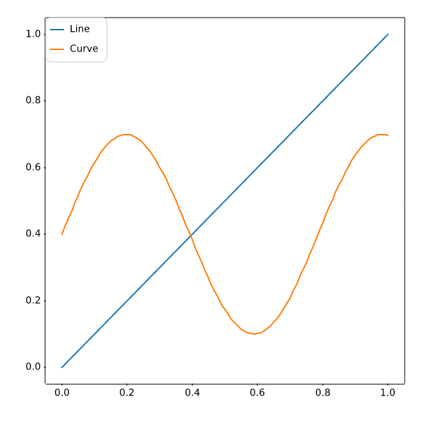
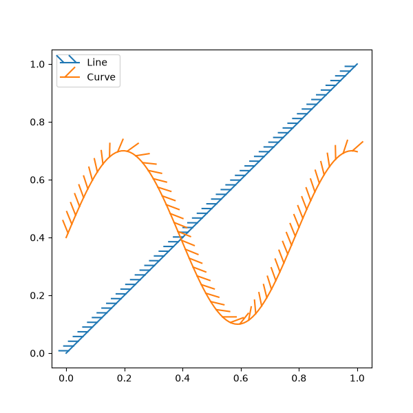
lines_bars_and_markers/linestyles
==========
Source
"""
==========
Linestyles
==========

Simple linestyles can be defined using the strings "solid", "dotted", "dashed"
or "dashdot". More refined control can be achieved by providing a dash tuple
``(offset, (on_off_seq))``. For example, ``(0, (3, 10, 1, 15))`` means
(3pt line, 10pt space, 1pt line, 15pt space) with no offset, while
``(5, (10, 3))``, means (10pt line, 3pt space), but skip the first 5pt line.
See also `.Line2D.set_linestyle`.  The specific on/off sequences of the
"dotted", "dashed" and "dashdot" styles are configurable:

* :rc:`lines.dotted_pattern`
* :rc:`lines.dashed_pattern`
* :rc:`lines.dashdot_pattern`

*Note*: The dash style can also be configured via `.Line2D.set_dashes`
as shown in :doc:`/gallery/lines_bars_and_markers/line_demo_dash_control`
and passing a list of dash sequences using the keyword *dashes* to the
cycler in :ref:`property_cycle <color_cycle>`.
"""
import matplotlib.pyplot as plt
import numpy as np

linestyle_str = [
     ('solid', 'solid'),      # Same as (0, ()) or '-'
     ('dotted', 'dotted'),    # Same as ':'
     ('dashed', 'dashed'),    # Same as '--'
     ('dashdot', 'dashdot')]  # Same as '-.'

linestyle_tuple = [
     ('loosely dotted',        (0, (1, 10))),
     ('dotted',                (0, (1, 5))),
     ('densely dotted',        (0, (1, 1))),

     ('long dash with offset', (5, (10, 3))),
     ('loosely dashed',        (0, (5, 10))),
     ('dashed',                (0, (5, 5))),
     ('densely dashed',        (0, (5, 1))),

     ('loosely dashdotted',    (0, (3, 10, 1, 10))),
     ('dashdotted',            (0, (3, 5, 1, 5))),
     ('densely dashdotted',    (0, (3, 1, 1, 1))),

     ('dashdotdotted',         (0, (3, 5, 1, 5, 1, 5))),
     ('loosely dashdotdotted', (0, (3, 10, 1, 10, 1, 10))),
     ('densely dashdotdotted', (0, (3, 1, 1, 1, 1, 1)))]


def plot_linestyles(ax, linestyles, title):
    X, Y = np.linspace(0, 100, 10), np.zeros(10)
    yticklabels = []

    for i, (name, linestyle) in enumerate(linestyles):
        ax.plot(X, Y+i, linestyle=linestyle, linewidth=1.5, color='black')
        yticklabels.append(name)

    ax.set_title(title)
    ax.set(ylim=(-0.5, len(linestyles)-0.5),
           yticks=np.arange(len(linestyles)),
           yticklabels=yticklabels)
    ax.tick_params(left=False, bottom=False, labelbottom=False)
    ax.spines[:].set_visible(False)

    # For each line style, add a text annotation with a small offset from
    # the reference point (0 in Axes coords, y tick value in Data coords).
    for i, (name, linestyle) in enumerate(linestyles):
        ax.annotate(repr(linestyle),
                    xy=(0.0, i), xycoords=ax.get_yaxis_transform(),
                    xytext=(-6, -12), textcoords='offset points',
                    color="blue", fontsize=8, ha="right", family="monospace")


fig, (ax0, ax1) = plt.subplots(2, 1, figsize=(7, 8), height_ratios=[1, 3],
                               layout='constrained')

plot_linestyles(ax0, linestyle_str[::-1], title='Named linestyles')
plot_linestyles(ax1, linestyle_tuple[::-1], title='Parametrized linestyles')

plt.show()

# %%
# .. tags::
#
#    styling: linestyle
#    purpose: reference
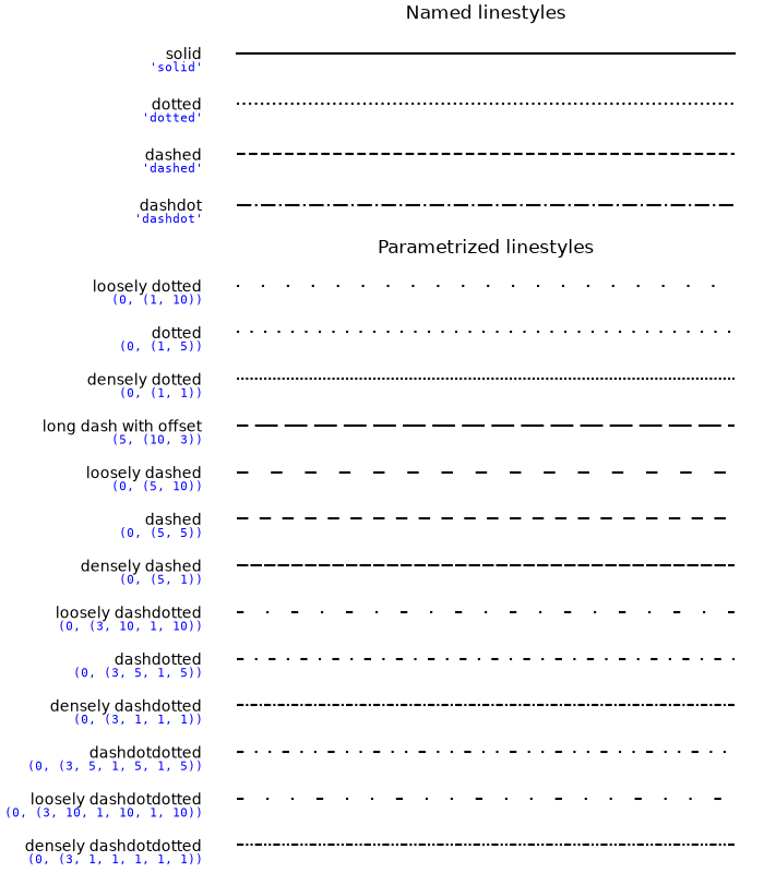
lines_bars_and_markers/marker_reference
================
Source
"""
================
Marker reference
================

Matplotlib supports multiple categories of markers which are selected using
the ``marker`` parameter of plot commands:

- `Unfilled markers`_
- `Filled markers`_
- `Markers created from TeX symbols`_
- `Markers created from Paths`_

For a list of all markers see also the `matplotlib.markers` documentation.

For example usages see
:doc:`/gallery/lines_bars_and_markers/scatter_star_poly`.

.. redirect-from:: /gallery/shapes_and_collections/marker_path
"""

import matplotlib.pyplot as plt

from matplotlib.lines import Line2D
from matplotlib.markers import MarkerStyle
from matplotlib.transforms import Affine2D

text_style = dict(horizontalalignment='right', verticalalignment='center',
                  fontsize=12, fontfamily='monospace')
marker_style = dict(linestyle=':', color='0.8', markersize=10,
                    markerfacecolor="tab:blue", markeredgecolor="tab:blue")


def format_axes(ax):
    ax.margins(0.2)
    ax.set_axis_off()
    ax.invert_yaxis()


def split_list(a_list):
    i_half = len(a_list) // 2
    return a_list[:i_half], a_list[i_half:]


# %%
# Unfilled markers
# ================
# Unfilled markers are single-colored.

fig, axs = plt.subplots(ncols=2)
fig.suptitle('Un-filled markers', fontsize=14)

# Filter out filled markers and marker settings that do nothing.
unfilled_markers = [m for m, func in Line2D.markers.items()
                    if func != 'nothing' and m not in Line2D.filled_markers]

for ax, markers in zip(axs, split_list(unfilled_markers)):
    for y, marker in enumerate(markers):
        ax.text(-0.5, y, repr(marker), **text_style)
        ax.plot([y] * 3, marker=marker, **marker_style)
    format_axes(ax)

# %%
# Filled markers
# ==============

fig, axs = plt.subplots(ncols=2)
fig.suptitle('Filled markers', fontsize=14)
for ax, markers in zip(axs, split_list(Line2D.filled_markers)):
    for y, marker in enumerate(markers):
        ax.text(-0.5, y, repr(marker), **text_style)
        ax.plot([y] * 3, marker=marker, **marker_style)
    format_axes(ax)

# %%
# .. _marker_fill_styles:
#
# Marker fill styles
# ------------------
# The edge color and fill color of filled markers can be specified separately.
# Additionally, the ``fillstyle`` can be configured to be unfilled, fully
# filled, or half-filled in various directions. The half-filled styles use
# ``markerfacecoloralt`` as secondary fill color.

fig, ax = plt.subplots()
fig.suptitle('Marker fillstyle', fontsize=14)
fig.subplots_adjust(left=0.4)

filled_marker_style = dict(marker='o', linestyle=':', markersize=15,
                           color='darkgrey',
                           markerfacecolor='tab:blue',
                           markerfacecoloralt='lightsteelblue',
                           markeredgecolor='brown')

for y, fill_style in enumerate(Line2D.fillStyles):
    ax.text(-0.5, y, repr(fill_style), **text_style)
    ax.plot([y] * 3, fillstyle=fill_style, **filled_marker_style)
format_axes(ax)

# %%
# Markers created from TeX symbols
# ================================
#
# Use :ref:`MathText <mathtext>`, to use custom marker symbols,
# like e.g. ``"$\u266B$"``. For an overview over the STIX font symbols refer
# to the `STIX font table <http://www.stixfonts.org/allGlyphs.html>`_.
# Also see the :doc:`/gallery/text_labels_and_annotations/stix_fonts_demo`.


fig, ax = plt.subplots()
fig.suptitle('Mathtext markers', fontsize=14)
fig.subplots_adjust(left=0.4)

marker_style.update(markeredgecolor="none", markersize=15)
markers = ["$1$", r"$\frac{1}{2}$", "$f$", "$\u266B$", r"$\mathcal{A}$"]

for y, marker in enumerate(markers):
    # Escape dollars so that the text is written "as is", not as mathtext.
    ax.text(-0.5, y, repr(marker).replace("$", r"\$"), **text_style)
    ax.plot([y] * 3, marker=marker, **marker_style)
format_axes(ax)

# %%
# Markers created from Paths
# ==========================
#
# Any `~.path.Path` can be used as a marker. The following example shows two
# simple paths *star* and *circle*, and a more elaborate path of a circle with
# a cut-out star.

import numpy as np

import matplotlib.path as mpath

star = mpath.Path.unit_regular_star(6)
circle = mpath.Path.unit_circle()
# concatenate the circle with an internal cutout of the star
cut_star = mpath.Path(
    vertices=np.concatenate([circle.vertices, star.vertices[::-1, ...]]),
    codes=np.concatenate([circle.codes, star.codes]))

fig, ax = plt.subplots()
fig.suptitle('Path markers', fontsize=14)
fig.subplots_adjust(left=0.4)

markers = {'star': star, 'circle': circle, 'cut_star': cut_star}

for y, (name, marker) in enumerate(markers.items()):
    ax.text(-0.5, y, name, **text_style)
    ax.plot([y] * 3, marker=marker, **marker_style)
format_axes(ax)

# %%
# Advanced marker modifications with transform
# ============================================
#
# Markers can be modified by passing a transform to the MarkerStyle
# constructor. Following example shows how a supplied rotation is applied to
# several marker shapes.

common_style = {k: v for k, v in filled_marker_style.items() if k != 'marker'}
angles = [0, 10, 20, 30, 45, 60, 90]

fig, ax = plt.subplots()
fig.suptitle('Rotated markers', fontsize=14)

ax.text(-0.5, 0, 'Filled marker', **text_style)
for x, theta in enumerate(angles):
    t = Affine2D().rotate_deg(theta)
    ax.plot(x, 0, marker=MarkerStyle('o', 'left', t), **common_style)

ax.text(-0.5, 1, 'Un-filled marker', **text_style)
for x, theta in enumerate(angles):
    t = Affine2D().rotate_deg(theta)
    ax.plot(x, 1, marker=MarkerStyle('1', 'left', t), **common_style)

ax.text(-0.5, 2, 'Equation marker', **text_style)
for x, theta in enumerate(angles):
    t = Affine2D().rotate_deg(theta)
    eq = r'$\frac{1}{x}$'
    ax.plot(x, 2, marker=MarkerStyle(eq, 'left', t), **common_style)

for x, theta in enumerate(angles):
    ax.text(x, 2.5, f"{theta}°", horizontalalignment="center")
format_axes(ax)

fig.tight_layout()

# %%
# Setting marker cap style and join style
# =======================================
#
# Markers have default cap and join styles, but these can be
# customized when creating a MarkerStyle.

from matplotlib.markers import CapStyle, JoinStyle

marker_inner = dict(markersize=35,
                    markerfacecolor='tab:blue',
                    markerfacecoloralt='lightsteelblue',
                    markeredgecolor='brown',
                    markeredgewidth=8,
                    )

marker_outer = dict(markersize=35,
                    markerfacecolor='tab:blue',
                    markerfacecoloralt='lightsteelblue',
                    markeredgecolor='white',
                    markeredgewidth=1,
                    )

fig, ax = plt.subplots()
fig.suptitle('Marker CapStyle', fontsize=14)
fig.subplots_adjust(left=0.1)

for y, cap_style in enumerate(CapStyle):
    ax.text(-0.5, y, cap_style.name, **text_style)
    for x, theta in enumerate(angles):
        t = Affine2D().rotate_deg(theta)
        m = MarkerStyle('1', transform=t, capstyle=cap_style)
        ax.plot(x, y, marker=m, **marker_inner)
        ax.plot(x, y, marker=m, **marker_outer)
        ax.text(x, len(CapStyle) - .5, f'{theta}°', ha='center')
format_axes(ax)

# %%
# Modifying the join style:

fig, ax = plt.subplots()
fig.suptitle('Marker JoinStyle', fontsize=14)
fig.subplots_adjust(left=0.05)

for y, join_style in enumerate(JoinStyle):
    ax.text(-0.5, y, join_style.name, **text_style)
    for x, theta in enumerate(angles):
        t = Affine2D().rotate_deg(theta)
        m = MarkerStyle('*', transform=t, joinstyle=join_style)
        ax.plot(x, y, marker=m, **marker_inner)
        ax.text(x, len(JoinStyle) - .5, f'{theta}°', ha='center')
format_axes(ax)

plt.show()

# %%
# .. tags::
#
#    component: marker
#    purpose: reference
lines_bars_and_markers/markevery_demo
==============
Source
"""
==============
Markevery Demo
==============

The ``markevery`` property of `.Line2D` allows drawing markers at a subset of
data points.

The list of possible parameters is specified at `.Line2D.set_markevery`.
In short:

- A single integer N draws every N-th marker.
- A tuple of integers (start, N) draws every N-th marker, starting at data
  index *start*.
- A list of integers draws the markers at the specified indices.
- A slice draws the markers at the sliced indices.
- A float specifies the distance between markers as a fraction of the Axes
  diagonal in screen space. This will lead to a visually uniform distribution
  of the points along the line, irrespective of scales and zooming.
"""

import matplotlib.pyplot as plt
import numpy as np

# define a list of markevery cases to plot
cases = [
    None,
    8,
    (30, 8),
    [16, 24, 32],
    [0, -1],
    slice(100, 200, 3),
    0.1,
    0.4,
    (0.2, 0.4)
]

# data points
delta = 0.11
x = np.linspace(0, 10 - 2 * delta, 200) + delta
y = np.sin(x) + 1.0 + delta

# %%
# markevery with linear scales
# ----------------------------

fig, axs = plt.subplots(3, 3, figsize=(10, 6), layout='constrained')
for ax, markevery in zip(axs.flat, cases):
    ax.set_title(f'markevery={markevery}')
    ax.plot(x, y, 'o', ls='-', ms=4, markevery=markevery)

# %%
# markevery with log scales
# -------------------------
#
# Note that the log scale causes a visual asymmetry in the marker distance for
# when subsampling the data using an integer. In contrast, subsampling on
# fraction of figure size creates even distributions, because it's based on
# fractions of the Axes diagonal, not on data coordinates or data indices.

fig, axs = plt.subplots(3, 3, figsize=(10, 6), layout='constrained')
for ax, markevery in zip(axs.flat, cases):
    ax.set_title(f'markevery={markevery}')
    ax.set_xscale('log')
    ax.set_yscale('log')
    ax.plot(x, y, 'o', ls='-', ms=4, markevery=markevery)

# %%
# markevery on zoomed plots
# -------------------------
#
# Integer-based *markevery* specifications select points from the underlying
# data and are independent on the view. In contrast, float-based specifications
# are related to the Axes diagonal. While zooming does not change the Axes
# diagonal, it changes the displayed data range, and more points will be
# displayed when zooming.

fig, axs = plt.subplots(3, 3, figsize=(10, 6), layout='constrained')
for ax, markevery in zip(axs.flat, cases):
    ax.set_title(f'markevery={markevery}')
    ax.plot(x, y, 'o', ls='-', ms=4, markevery=markevery)
    ax.set_xlim(6, 6.7)
    ax.set_ylim(1.1, 1.7)

# %%
# markevery on polar plots
# ------------------------

r = np.linspace(0, 3.0, 200)
theta = 2 * np.pi * r

fig, axs = plt.subplots(3, 3, figsize=(10, 6), layout='constrained',
                        subplot_kw={'projection': 'polar'})
for ax, markevery in zip(axs.flat, cases):
    ax.set_title(f'markevery={markevery}')
    ax.plot(theta, r, 'o', ls='-', ms=4, markevery=markevery)

plt.show()

# %%
# .. tags::
#
#    component: marker
#    plot-type: line
#    level: beginner
lines_bars_and_markers/masked_demo
==============================
Source
"""
==============================
Plotting masked and NaN values
==============================

Sometimes you need to plot data with missing values.

One possibility is to simply remove undesired data points. The line plotted
through the remaining data will be continuous, and not indicate where the
missing data is located.

If it is useful to have gaps in the line where the data is missing, then the
undesired points can be indicated using a `masked array`_ or by setting their
values to NaN. No marker will be drawn where either x or y are masked and, if
plotting with a line, it will be broken there.

.. _masked array:
   https://numpy.org/doc/stable/reference/maskedarray.generic.html

The following example illustrates the three cases:

1) Removing points.
2) Masking points.
3) Setting to NaN.
"""

import matplotlib.pyplot as plt
import numpy as np

x = np.linspace(-np.pi/2, np.pi/2, 31)
y = np.cos(x)**3

# 1) remove points where y > 0.7
x2 = x[y <= 0.7]
y2 = y[y <= 0.7]

# 2) mask points where y > 0.7
y3 = np.ma.masked_where(y > 0.7, y)

# 3) set to NaN where y > 0.7
y4 = y.copy()
y4[y3 > 0.7] = np.nan

plt.plot(x*0.1, y, 'o-', color='lightgrey', label='No mask')
plt.plot(x2*0.4, y2, 'o-', label='Points removed')
plt.plot(x*0.7, y3, 'o-', label='Masked values')
plt.plot(x*1.0, y4, 'o-', label='NaN values')
plt.legend()
plt.title('Masked and NaN data')
plt.show()

# %%
# .. tags::
#
#    plot-type: line
#    level: intermediate
lines_bars_and_markers/multicolored_line
==================
Source
"""
==================
Multicolored lines
==================

The example shows two ways to plot a line with the a varying color defined by
a third value. The first example defines the color at each (x, y) point.
The second example defines the color between pairs of points, so the length
of the color value list is one less than the length of the x and y lists.

Color values at points
----------------------

"""

import warnings

import matplotlib.pyplot as plt
import numpy as np

from matplotlib.collections import LineCollection


def colored_line(x, y, c, ax=None, **lc_kwargs):
    """
    Plot a line with a color specified along the line by a third value.

    It does this by creating a collection of line segments. Each line segment is
    made up of two straight lines each connecting the current (x, y) point to the
    midpoints of the lines connecting the current point with its two neighbors.
    This creates a smooth line with no gaps between the line segments.

    Parameters
    ----------
    x, y : array-like
        The horizontal and vertical coordinates of the data points.
    c : array-like
        The color values, which should be the same size as x and y.
    ax : matplotlib.axes.Axes, optional
        The axes to plot on. If not provided, the current axes will be used.
    **lc_kwargs
        Any additional arguments to pass to matplotlib.collections.LineCollection
        constructor. This should not include the array keyword argument because
        that is set to the color argument. If provided, it will be overridden.

    Returns
    -------
    matplotlib.collections.LineCollection
        The generated line collection representing the colored line.
    """
    if "array" in lc_kwargs:
        warnings.warn(
            'The provided "array" keyword argument will be overridden',
            UserWarning,
            stacklevel=2,
        )

    xy = np.stack((x, y), axis=-1)
    xy_mid = np.concat(
        (xy[0, :][None, :], (xy[:-1, :] + xy[1:, :]) / 2, xy[-1, :][None, :]), axis=0
    )
    segments = np.stack((xy_mid[:-1, :], xy, xy_mid[1:, :]), axis=-2)
    # Note that
    # segments[0, :, :] is [xy[0, :], xy[0, :], (xy[0, :] + xy[1, :]) / 2]
    # segments[i, :, :] is [(xy[i - 1, :] + xy[i, :]) / 2, xy[i, :],
    #     (xy[i, :] + xy[i + 1, :]) / 2] if i not in {0, len(x) - 1}
    # segments[-1, :, :] is [(xy[-2, :] + xy[-1, :]) / 2, xy[-1, :], xy[-1, :]]

    lc_kwargs["array"] = c
    lc = LineCollection(segments, **lc_kwargs)

    # Plot the line collection to the axes
    ax = ax or plt.gca()
    ax.add_collection(lc)

    return lc


# -------------- Create and show plot --------------
# Some arbitrary function that gives x, y, and color values
t = np.linspace(-7.4, -0.5, 200)
x = 0.9 * np.sin(t)
y = 0.9 * np.cos(1.6 * t)
color = np.linspace(0, 2, t.size)

# Create a figure and plot the line on it
fig1, ax1 = plt.subplots()
lines = colored_line(x, y, color, ax1, linewidth=10, cmap="plasma")
fig1.colorbar(lines)  # add a color legend

ax1.set_title("Color at each point")

plt.show()

####################################################################
# This method is designed to give a smooth impression when distances and color
# differences between adjacent points are not too large. The following example
# does not meet this criteria and by that serves to illustrate the segmentation
# and coloring mechanism.
x = [0, 1, 2, 3, 4]
y = [0, 1, 2, 1, 1]
c = [1, 2, 3, 4, 5]
fig, ax = plt.subplots()
ax.scatter(x, y, c=c, cmap='rainbow')
colored_line(x, y, c=c, ax=ax, cmap='rainbow')

plt.show()

####################################################################
# Color values between points
# ---------------------------
#


def colored_line_between_pts(x, y, c, ax, **lc_kwargs):
    """
    Plot a line with a color specified between (x, y) points by a third value.

    It does this by creating a collection of line segments between each pair of
    neighboring points. The color of each segment is determined by the
    made up of two straight lines each connecting the current (x, y) point to the
    midpoints of the lines connecting the current point with its two neighbors.
    This creates a smooth line with no gaps between the line segments.

    Parameters
    ----------
    x, y : array-like
        The horizontal and vertical coordinates of the data points.
    c : array-like
        The color values, which should have a size one less than that of x and y.
    ax : Axes
        Axis object on which to plot the colored line.
    **lc_kwargs
        Any additional arguments to pass to matplotlib.collections.LineCollection
        constructor. This should not include the array keyword argument because
        that is set to the color argument. If provided, it will be overridden.

    Returns
    -------
    matplotlib.collections.LineCollection
        The generated line collection representing the colored line.
    """
    if "array" in lc_kwargs:
        warnings.warn('The provided "array" keyword argument will be overridden')

    # Check color array size (LineCollection still works, but values are unused)
    if len(c) != len(x) - 1:
        warnings.warn(
            "The c argument should have a length one less than the length of x and y. "
            "If it has the same length, use the colored_line function instead."
        )

    # Create a set of line segments so that we can color them individually
    # This creates the points as an N x 1 x 2 array so that we can stack points
    # together easily to get the segments. The segments array for line collection
    # needs to be (numlines) x (points per line) x 2 (for x and y)
    points = np.array([x, y]).T.reshape(-1, 1, 2)
    segments = np.concatenate([points[:-1], points[1:]], axis=1)
    lc = LineCollection(segments, **lc_kwargs)

    # Set the values used for colormapping
    lc.set_array(c)

    return ax.add_collection(lc)


# -------------- Create and show plot --------------
x = np.linspace(0, 3 * np.pi, 500)
y = np.sin(x)
dydx = np.cos(0.5 * (x[:-1] + x[1:]))  # first derivative

fig2, ax2 = plt.subplots()
line = colored_line_between_pts(x, y, dydx, ax2, linewidth=2, cmap="viridis")
fig2.colorbar(line, ax=ax2, label="dy/dx")

ax2.set_xlim(x.min(), x.max())
ax2.set_ylim(-1.1, 1.1)
ax2.set_title("Color between points")

plt.show()

# %%
# .. tags::
#
#    styling: color
#    styling: linestyle
#    plot-type: line
#    level: intermediate
lines_bars_and_markers/multivariate_marker_plot
==============================================
Source
"""
==============================================
Mapping marker properties to multivariate data
==============================================

This example shows how to use different properties of markers to plot
multivariate datasets. Here we represent a successful baseball throw as a
smiley face with marker size mapped to the skill of thrower, marker rotation to
the take-off angle, and thrust to the marker color.
"""

import matplotlib.pyplot as plt
import numpy as np

from matplotlib.colors import Normalize
from matplotlib.markers import MarkerStyle
from matplotlib.text import TextPath
from matplotlib.transforms import Affine2D

SUCCESS_SYMBOLS = [
    TextPath((0, 0), "☹"),
    TextPath((0, 0), "😒"),
    TextPath((0, 0), "☺"),
]

N = 25
np.random.seed(42)
skills = np.random.uniform(5, 80, size=N) * 0.1 + 5
takeoff_angles = np.random.normal(0, 90, N)
thrusts = np.random.uniform(size=N)
successful = np.random.randint(0, 3, size=N)
positions = np.random.normal(size=(N, 2)) * 5
data = zip(skills, takeoff_angles, thrusts, successful, positions)

cmap = plt.colormaps["plasma"]
fig, ax = plt.subplots()
fig.suptitle("Throwing success", size=14)
for skill, takeoff, thrust, mood, pos in data:
    t = Affine2D().scale(skill).rotate_deg(takeoff)
    m = MarkerStyle(SUCCESS_SYMBOLS[mood], transform=t)
    ax.plot(pos[0], pos[1], marker=m, color=cmap(thrust))
fig.colorbar(plt.cm.ScalarMappable(norm=Normalize(0, 1), cmap="plasma"),
             ax=ax, label="Normalized Thrust [a.u.]")
ax.set_xlabel("X position [m]")
ax.set_ylabel("Y position [m]")

plt.show()

# %%
# .. tags::
#
#    component: marker
#    styling: color,
#    styling: shape
#    level: beginner
#    purpose: fun
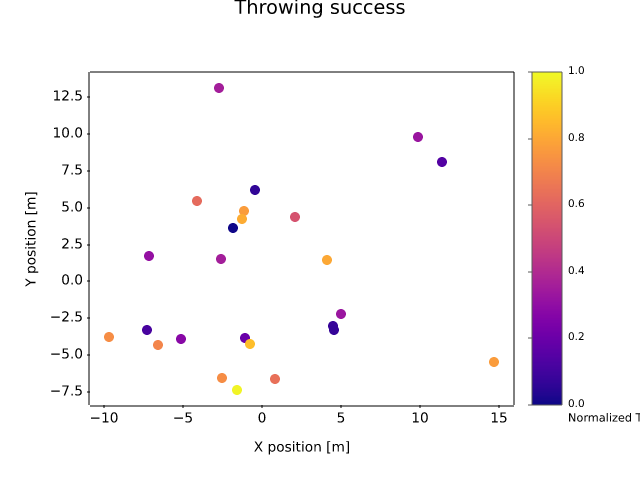
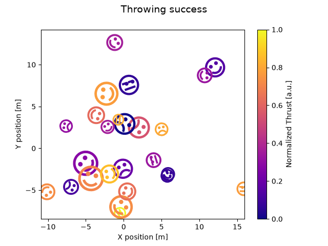
lines_bars_and_markers/scatter_demo2
=============
Source
"""
=============
Scatter Demo2
=============

Demo of scatter plot with varying marker colors and sizes.
"""
import matplotlib.pyplot as plt
import numpy as np

import matplotlib.cbook as cbook

# Load a numpy record array from yahoo csv data with fields date, open, high,
# low, close, volume, adj_close from the mpl-data/sample_data directory. The
# record array stores the date as an np.datetime64 with a day unit ('D') in
# the date column.
price_data = cbook.get_sample_data('goog.npz')['price_data']
price_data = price_data[-250:]  # get the most recent 250 trading days

delta1 = np.diff(price_data["adj_close"]) / price_data["adj_close"][:-1]

# Marker size in units of points^2
volume = (15 * price_data["volume"][:-2] / price_data["volume"][0])**2
close = 0.003 * price_data["close"][:-2] / 0.003 * price_data["open"][:-2]

fig, ax = plt.subplots()
ax.scatter(delta1[:-1], delta1[1:], c=close, s=volume, alpha=0.5)

ax.set_xlabel(r'$\Delta_i$', fontsize=15)
ax.set_ylabel(r'$\Delta_{i+1}$', fontsize=15)
ax.set_title('Volume and percent change')

ax.grid(True)
fig.tight_layout()

plt.show()

# %%
# .. tags::
#
#    component: marker
#    styling: color
#    styling: colormap
#    plot-type: scatter
#    level: beginner
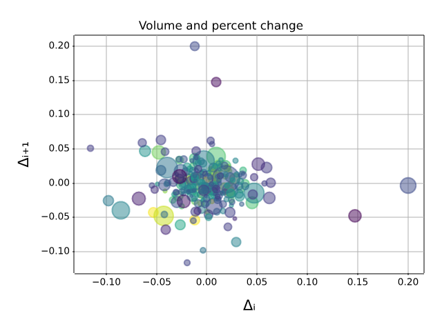
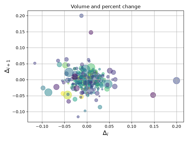
lines_bars_and_markers/scatter_hist
============================
Source
"""
============================
Scatter plot with histograms
============================

Add histograms to the x-axes and y-axes margins of a scatter plot.

This layout features a central scatter plot illustrating the relationship
between x and y, a histogram at the top displaying the distribution of x, and a
histogram on the right showing the distribution of y.

For a nice alignment of the main Axes with the marginals, two options are shown
below:

.. contents::
   :local:

While `.Axes.inset_axes` may be a bit more complex, it allows correct handling
of main Axes with a fixed aspect ratio.

Let us first define a function that takes x and y data as input, as well as
three Axes, the main Axes for the scatter, and two marginal Axes. It will then
create the scatter and histograms inside the provided Axes.
"""

import matplotlib.pyplot as plt
import numpy as np

# Fixing random state for reproducibility
np.random.seed(19680801)

# some random data
x = np.random.randn(1000)
y = np.random.randn(1000)


def scatter_hist(x, y, ax, ax_histx, ax_histy):
    # no labels
    ax_histx.tick_params(axis="x", labelbottom=False)
    ax_histy.tick_params(axis="y", labelleft=False)

    # the scatter plot:
    ax.scatter(x, y)

    # now determine nice limits by hand:
    binwidth = 0.25
    xymax = max(np.max(np.abs(x)), np.max(np.abs(y)))
    lim = (int(xymax/binwidth) + 1) * binwidth

    bins = np.arange(-lim, lim + binwidth, binwidth)
    ax_histx.hist(x, bins=bins)
    ax_histy.hist(y, bins=bins, orientation='horizontal')


# %%
# Defining the Axes positions using subplot_mosaic
# ------------------------------------------------
#
# We use the `~.pyplot.subplot_mosaic` function to define the positions and
# names of the three axes; the empty axes is specified by ``'.'``.  We manually
# specify the size of the figure, and can make the different axes have
# different sizes by specifying the *width_ratios* and *height_ratios*
# arguments. The *layout* argument is set to ``'constrained'`` to optimize the
# spacing between the axes.

fig, axs = plt.subplot_mosaic([['histx', '.'],
                               ['scatter', 'histy']],
                              figsize=(6, 6),
                              width_ratios=(4, 1), height_ratios=(1, 4),
                              layout='constrained')
scatter_hist(x, y, axs['scatter'], axs['histx'], axs['histy'])


# %%
#
# Defining the Axes positions using inset_axes
# --------------------------------------------
#
# `~.Axes.inset_axes` can be used to position marginals *outside* the main
# Axes.  The advantage of doing so is that the aspect ratio of the main Axes
# can be fixed, and the marginals will always be drawn relative to the position
# of the Axes.

# Create a Figure, which doesn't have to be square.
fig = plt.figure(layout='constrained')
# Create the main Axes.
ax = fig.add_subplot()
# The main Axes' aspect can be fixed.
ax.set_aspect('equal')
# Create marginal Axes, which have 25% of the size of the main Axes.  Note that
# the inset Axes are positioned *outside* (on the right and the top) of the
# main Axes, by specifying axes coordinates greater than 1.  Axes coordinates
# less than 0 would likewise specify positions on the left and the bottom of
# the main Axes.
ax_histx = ax.inset_axes([0, 1.05, 1, 0.25], sharex=ax)
ax_histy = ax.inset_axes([1.05, 0, 0.25, 1], sharey=ax)
# Draw the scatter plot and marginals.
scatter_hist(x, y, ax, ax_histx, ax_histy)

plt.show()


# %%
#
# While we recommend using one of the two methods described above, there are
# number of other ways to achieve a similar layout:
#
# - The Axes can be positioned manually in relative coordinates using
#   `~matplotlib.figure.Figure.add_axes`.
# - A gridspec can be used to create the layout
#   (`~matplotlib.figure.Figure.add_gridspec`) and adding only the three desired
#   axes (`~matplotlib.figure.Figure.add_subplot`).
# - Four subplots can be created  using `~.pyplot.subplots`,  and the unused
#   axes in the upper right can be removed manually.
# - The ``axes_grid1`` toolkit can be used, as shown in
#   :doc:`/gallery/axes_grid1/scatter_hist_locatable_axes`.
#
# .. admonition:: References
#
#    The use of the following functions, methods, classes and modules is shown
#    in this example:
#
#    - `matplotlib.figure.Figure.subplot_mosaic`
#    - `matplotlib.pyplot.subplot_mosaic`
#    - `matplotlib.figure.Figure.add_subplot`
#    - `matplotlib.axes.Axes.inset_axes`
#    - `matplotlib.axes.Axes.scatter`
#    - `matplotlib.axes.Axes.hist`
#
# .. tags::
#
#    component: axes
#    plot-type: scatter
#    plot-type: histogram
#    level: intermediate
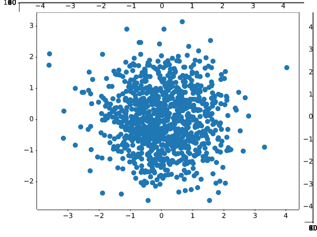
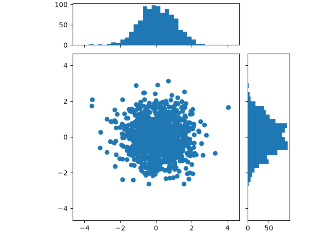
lines_bars_and_markers/scatter_masked
===============================
Source
"""
===============================
Scatter plot with masked values
===============================

Mask some data points and add a line demarking
masked regions.

"""
import matplotlib.pyplot as plt
import numpy as np

# Fixing random state for reproducibility
np.random.seed(19680801)


N = 100
r0 = 0.6
x = 0.9 * np.random.rand(N)
y = 0.9 * np.random.rand(N)
area = (20 * np.random.rand(N))**2  # 0 to 10 point radii
c = np.sqrt(area)
r = np.sqrt(x ** 2 + y ** 2)
area1 = np.ma.masked_where(r < r0, area)
area2 = np.ma.masked_where(r >= r0, area)
plt.scatter(x, y, s=area1, marker='^', c=c)
plt.scatter(x, y, s=area2, marker='o', c=c)
# Show the boundary between the regions:
theta = np.arange(0, np.pi / 2, 0.01)
plt.plot(r0 * np.cos(theta), r0 * np.sin(theta))

plt.show()

# %%
# .. tags::
#
#    component: marker
#    plot-type: scatter
#    level: beginner
lines_bars_and_markers/scatter_star_poly
===============
Source
"""
===============
Marker examples
===============

Demonstrates several ways to specify markers in scatter plots,
including built-in marker styles and custom marker paths.

See also the `matplotlib.markers` documentation for a list of all markers and
:doc:`/gallery/lines_bars_and_markers/marker_reference` for more information
on configuring markers.

.. redirect-from:: /gallery/lines_bars_and_markers/scatter_custom_symbol
.. redirect-from:: /gallery/lines_bars_and_markers/scatter_symbol
.. redirect-from:: /gallery/lines_bars_and_markers/scatter_piecharts
"""
import matplotlib.pyplot as plt
import numpy as np

# Fixing random state for reproducibility
np.random.seed(19680801)

x = np.random.rand(10)
y = np.random.rand(10)
z = np.sqrt(x**2 + y**2)

fig, axs = plt.subplots(2, 3, sharex=True, sharey=True, layout="constrained")

# Matplotlib marker symbol
axs[0, 0].scatter(x, y, s=80, c=z, marker=">")
axs[0, 0].set_title("marker='>'")

# marker from TeX: passing a TeX symbol name enclosed in $-signs
axs[0, 1].scatter(x, y, s=80, c=z, marker=r"$\clubsuit$")
axs[0, 1].set_title(r"marker=r'\$\clubsuit\$'")

# marker from path: passing a custom path of N vertices as a (N, 2) array-like
verts = [[-1, -1], [1, -1], [1, 1], [-1, -1]]
axs[0, 2].scatter(x, y, s=80, c=z, marker=verts)
axs[0, 2].set_title("marker=verts")

# regular pentagon marker
axs[1, 0].scatter(x, y, s=80, c=z, marker=(5, 0))
axs[1, 0].set_title("marker=(5, 0)")

# regular 5-pointed star marker
axs[1, 1].scatter(x, y, s=80, c=z, marker=(5, 1))
axs[1, 1].set_title("marker=(5, 1)")

# regular 5-pointed asterisk marker
axs[1, 2].scatter(x, y, s=80, c=z, marker=(5, 2))
axs[1, 2].set_title("marker=(5, 2)")

plt.show()

# %%
# .. tags::
#
#    component: marker
#    level: beginner
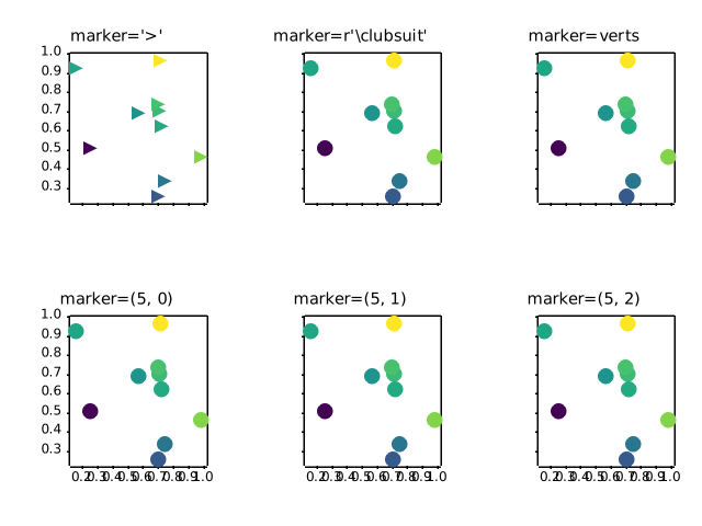
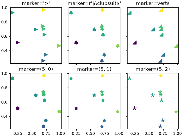
lines_bars_and_markers/scatter_with_legend
==========================
Source
"""
==========================
Scatter plot with a legend
==========================

To create a scatter plot with a legend one may use a loop and create one
`~.Axes.scatter` plot per item to appear in the legend and set the ``label``
accordingly.

The following also demonstrates how transparency of the markers
can be adjusted by giving ``alpha`` a value between 0 and 1.
"""

import matplotlib.pyplot as plt
import numpy as np

np.random.seed(19680801)


fig, ax = plt.subplots()
for color in ['tab:blue', 'tab:orange', 'tab:green']:
    n = 750
    x, y = np.random.rand(2, n)
    scale = 200.0 * np.random.rand(n)
    ax.scatter(x, y, c=color, s=scale, label=color,
               alpha=0.3, edgecolors='none')

ax.legend()
ax.grid(True)

plt.show()


# %%
# .. _automatedlegendcreation:
#
# Automated legend creation
# -------------------------
#
# Another option for creating a legend for a scatter is to use the
# `.PathCollection.legend_elements` method.  It will automatically try to
# determine a useful number of legend entries to be shown and return a tuple of
# handles and labels. Those can be passed to the call to `~.axes.Axes.legend`.


N = 45
x, y = np.random.rand(2, N)
c = np.random.randint(1, 5, size=N)
s = np.random.randint(10, 220, size=N)

fig, ax = plt.subplots()

scatter = ax.scatter(x, y, c=c, s=s)

# produce a legend with the unique colors from the scatter
legend1 = ax.legend(*scatter.legend_elements(),
                    loc="lower left", title="Classes")
ax.add_artist(legend1)

# produce a legend with a cross-section of sizes from the scatter
handles, labels = scatter.legend_elements(prop="sizes", alpha=0.6)
legend2 = ax.legend(handles, labels, loc="upper right", title="Sizes")

plt.show()


# %%
# Further arguments to the `.PathCollection.legend_elements` method
# can be used to steer how many legend entries are to be created and how they
# should be labeled. The following shows how to use some of them.

volume = np.random.rayleigh(27, size=40)
amount = np.random.poisson(10, size=40)
ranking = np.random.normal(size=40)
price = np.random.uniform(1, 10, size=40)

fig, ax = plt.subplots()

# Because the price is much too small when being provided as size for ``s``,
# we normalize it to some useful point sizes, s=0.3*(price*3)**2
scatter = ax.scatter(volume, amount, c=ranking, s=0.3*(price*3)**2,
                     vmin=-3, vmax=3, cmap="Spectral")

# Produce a legend for the ranking (colors). Even though there are 40 different
# rankings, we only want to show 5 of them in the legend.
legend1 = ax.legend(*scatter.legend_elements(num=5),
                    loc="upper left", title="Ranking")
ax.add_artist(legend1)

# Produce a legend for the price (sizes). Because we want to show the prices
# in dollars, we use the *func* argument to supply the inverse of the function
# used to calculate the sizes from above. The *fmt* ensures to show the price
# in dollars. Note how we target at 5 elements here, but obtain only 4 in the
# created legend due to the automatic round prices that are chosen for us.
kw = dict(prop="sizes", num=5, color=scatter.cmap(0.7), fmt="$ {x:.2f}",
          func=lambda s: np.sqrt(s/.3)/3)
legend2 = ax.legend(*scatter.legend_elements(**kw),
                    loc="lower right", title="Price")

plt.show()

# %%
#
# .. admonition:: References
#
#    The use of the following functions, methods, classes and modules is shown
#    in this example:
#
#    - `matplotlib.axes.Axes.scatter` / `matplotlib.pyplot.scatter`
#    - `matplotlib.axes.Axes.legend` / `matplotlib.pyplot.legend`
#    - `matplotlib.collections.PathCollection.legend_elements`
#
# .. tags::
#
#    component: legend
#    plot-type: scatter
#    level: intermediate
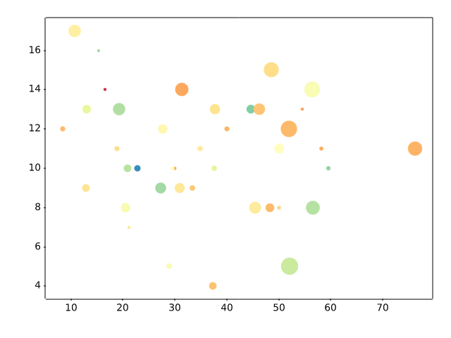
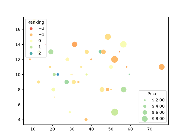
lines_bars_and_markers/simple_plot
=========
Source
"""
=========
Line plot
=========

Create a basic line plot.
"""

import matplotlib.pyplot as plt
import numpy as np

# Data for plotting
t = np.arange(0.0, 2.0, 0.01)
s = 1 + np.sin(2 * np.pi * t)

fig, ax = plt.subplots()
ax.plot(t, s)

ax.set(xlabel='time (s)', ylabel='voltage (mV)',
       title='About as simple as it gets, folks')
ax.grid()

fig.savefig("test.png")
plt.show()

# %%
#
# .. admonition:: References
#
#    The use of the following functions, methods, classes and modules is shown
#    in this example:
#
#    - `matplotlib.axes.Axes.plot` / `matplotlib.pyplot.plot`
#    - `matplotlib.pyplot.subplots`
#    - `matplotlib.figure.Figure.savefig`
#
# .. tags::
#
#    plot-type: line
#    level: beginner
lines_bars_and_markers/span_regions
==========================================================
Source
"""
==========================================================
Shade regions defined by a logical mask using fill_between
==========================================================
"""

import matplotlib.pyplot as plt
import numpy as np

t = np.arange(0.0, 2, 0.01)
s = np.sin(2*np.pi*t)

fig, ax = plt.subplots()

ax.plot(t, s, color='black')
ax.axhline(0, color='black')

ax.fill_between(t, 1, where=s > 0, facecolor='green', alpha=.5)
ax.fill_between(t, -1, where=s < 0, facecolor='red', alpha=.5)

plt.show()


# %%
#
# .. admonition:: References
#
#    The use of the following functions, methods, classes and modules is shown
#    in this example:
#
#    - `matplotlib.axes.Axes.fill_between`
#
# .. tags::
#
#    styling: conditional
#    plot-type: fill_between
#    level: beginner
lines_bars_and_markers/spectrum_demo
========================
Source
"""
========================
Spectrum representations
========================

The plots show different spectrum representations of a sine signal with
additive noise. A (frequency) spectrum of a discrete-time signal is calculated
by utilizing the fast Fourier transform (FFT).
"""
import matplotlib.pyplot as plt
import numpy as np

np.random.seed(0)

dt = 0.01  # sampling interval
Fs = 1 / dt  # sampling frequency
t = np.arange(0, 10, dt)

# generate noise:
nse = np.random.randn(len(t))
r = np.exp(-t / 0.05)
cnse = np.convolve(nse, r) * dt
cnse = cnse[:len(t)]

s = 0.1 * np.sin(4 * np.pi * t) + cnse  # the signal

fig = plt.figure(figsize=(7, 7), layout='constrained')
axs = fig.subplot_mosaic([["signal", "signal"],
                          ["magnitude", "log_magnitude"],
                          ["phase", "angle"]])

# plot time signal:
axs["signal"].set_title("Signal")
axs["signal"].plot(t, s, color='C0')
axs["signal"].set_xlabel("Time (s)")
axs["signal"].set_ylabel("Amplitude")

# plot different spectrum types:
axs["magnitude"].set_title("Magnitude Spectrum")
axs["magnitude"].magnitude_spectrum(s, Fs=Fs, color='C1')

axs["log_magnitude"].set_title("Log. Magnitude Spectrum")
axs["log_magnitude"].magnitude_spectrum(s, Fs=Fs, scale='dB', color='C1')

axs["phase"].set_title("Phase Spectrum ")
axs["phase"].phase_spectrum(s, Fs=Fs, color='C2')

axs["angle"].set_title("Angle Spectrum")
axs["angle"].angle_spectrum(s, Fs=Fs, color='C2')

plt.show()

# %%
# .. tags::
#
#    domain: signal-processing
#    plot-type: line
#    level: beginner
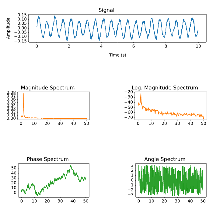
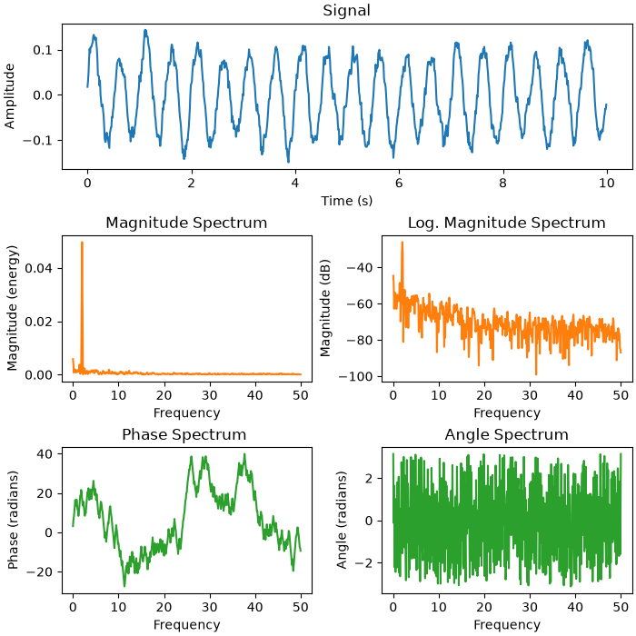
lines_bars_and_markers/stackplot_demo
===========================
Source
"""
===========================
Stackplots and streamgraphs
===========================
"""

# %%
# Stackplots
# ----------
#
# Stackplots draw multiple datasets as vertically stacked areas. This is
# useful when the individual data values and additionally their cumulative
# value are of interest.


import matplotlib.pyplot as plt
import numpy as np

import matplotlib.ticker as mticker

# data from United Nations World Population Prospects (Revision 2019)
# https://population.un.org/wpp/, license: CC BY 3.0 IGO
year = [1950, 1960, 1970, 1980, 1990, 2000, 2010, 2018]
population_by_continent = {
    'Africa': [.228, .284, .365, .477, .631, .814, 1.044, 1.275],
    'the Americas': [.340, .425, .519, .619, .727, .840, .943, 1.006],
    'Asia': [1.394, 1.686, 2.120, 2.625, 3.202, 3.714, 4.169, 4.560],
    'Europe': [.220, .253, .276, .295, .310, .303, .294, .293],
    'Oceania': [.012, .015, .019, .022, .026, .031, .036, .039],
}

fig, ax = plt.subplots()
ax.stackplot(year, population_by_continent.values(),
             labels=population_by_continent.keys(), alpha=0.8)
ax.legend(loc='upper left', reverse=True)
ax.set_title('World population')
ax.set_xlabel('Year')
ax.set_ylabel('Number of people (billions)')
# add tick at every 200 million people
ax.yaxis.set_minor_locator(mticker.MultipleLocator(.2))

plt.show()

# %%
# Streamgraphs
# ------------
#
# Using the *baseline* parameter, you can turn an ordinary stacked area plot
# with baseline 0 into a stream graph.


# Fixing random state for reproducibility
np.random.seed(19680801)


def gaussian_mixture(x, n=5):
    """Return a random mixture of *n* Gaussians, evaluated at positions *x*."""
    def add_random_gaussian(a):
        amplitude = 1 / (.1 + np.random.random())
        dx = x[-1] - x[0]
        x0 = (2 * np.random.random() - .5) * dx
        z = 10 / (.1 + np.random.random()) / dx
        a += amplitude * np.exp(-(z * (x - x0))**2)
    a = np.zeros_like(x)
    for j in range(n):
        add_random_gaussian(a)
    return a


x = np.linspace(0, 100, 101)
ys = [gaussian_mixture(x) for _ in range(3)]

fig, ax = plt.subplots()
ax.stackplot(x, ys, baseline='wiggle')
plt.show()

# %%
# .. tags::
#
#    plot-type: stackplot
#    level: intermediate
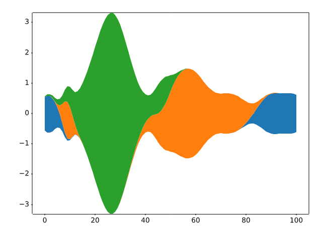
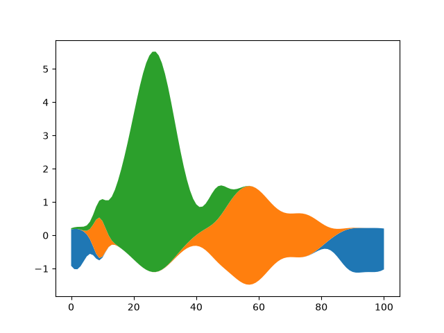
lines_bars_and_markers/stairs_demo
===========
Source
"""
===========
Stairs Demo
===========

This example demonstrates the use of `~.matplotlib.pyplot.stairs` for stepwise
constant functions. A common use case is histogram and histogram-like data
visualization.

"""

import matplotlib.pyplot as plt
import numpy as np

from matplotlib.patches import StepPatch

np.random.seed(0)
h, edges = np.histogram(np.random.normal(5, 3, 5000),
                        bins=np.linspace(0, 10, 20))

fig, axs = plt.subplots(3, 1, figsize=(7, 15))
axs[0].stairs(h, edges, label='Simple histogram')
axs[0].stairs(h, edges + 5, baseline=50, label='Modified baseline')
axs[0].stairs(h, edges + 10, baseline=None, label='No edges')
axs[0].set_title("Step Histograms")

axs[1].stairs(np.arange(1, 6, 1), fill=True,
              label='Filled histogram\nw/ automatic edges')
axs[1].stairs(np.arange(1, 6, 1)*0.3, np.arange(2, 8, 1),
              orientation='horizontal', hatch='//',
              label='Hatched histogram\nw/ horizontal orientation')
axs[1].set_title("Filled histogram")

patch = StepPatch(values=[1, 2, 3, 2, 1],
                  edges=range(1, 7),
                  label=('Patch derived underlying object\n'
                         'with default edge/facecolor behaviour'))
axs[2].add_patch(patch)
axs[2].set_xlim(0, 7)
axs[2].set_ylim(-1, 5)
axs[2].set_title("StepPatch artist")

for ax in axs:
    ax.legend()
plt.show()

# %%
# *baseline* can take an array to allow for stacked histogram plots
A = [[0, 0, 0],
     [1, 2, 3],
     [2, 4, 6],
     [3, 6, 9]]

for i in range(len(A) - 1):
    plt.stairs(A[i+1], baseline=A[i], fill=True)

# %%
# Comparison of `.pyplot.step` and `.pyplot.stairs`
# -------------------------------------------------
#
# `.pyplot.step` defines the positions of the steps as single values. The steps
# extend left/right/both ways from these reference values depending on the
# parameter *where*. The number of *x* and *y* values is the same.
#
# In contrast, `.pyplot.stairs` defines the positions of the steps via their
# bounds *edges*, which is one element longer than the step values.

bins = np.arange(14)
centers = bins[:-1] + np.diff(bins) / 2
y = np.sin(centers / 2)

plt.step(bins[:-1], y, where='post', label='step(where="post")')
plt.plot(bins[:-1], y, 'o--', color='grey', alpha=0.3)

plt.stairs(y - 1, bins, baseline=None, label='stairs()')
plt.plot(centers, y - 1, 'o--', color='grey', alpha=0.3)
plt.plot(np.repeat(bins, 2), np.hstack([y[0], np.repeat(y, 2), y[-1]]) - 1,
         'o', color='red', alpha=0.2)

plt.legend()
plt.title('step() vs. stairs()')
plt.show()

# %%
#
# .. admonition:: References
#
#    The use of the following functions, methods, classes and modules is shown
#    in this example:
#
#    - `matplotlib.axes.Axes.stairs` / `matplotlib.pyplot.stairs`
#    - `matplotlib.patches.StepPatch`
#
# .. tags::
#
#    plot-type: stairs
#    level: intermediate
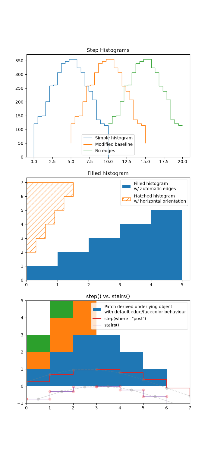
lines_bars_and_markers/stem_plot
=========
Source
"""
=========
Stem plot
=========

`~.pyplot.stem` plots vertical lines from a baseline to the y-coordinate and
places a marker at the tip.
"""
import matplotlib.pyplot as plt
import numpy as np

x = np.linspace(0.1, 2 * np.pi, 41)
y = np.exp(np.sin(x))

plt.stem(x, y)
plt.show()

# %%
#
# The position of the baseline can be adapted using *bottom*.
# The parameters *linefmt*, *markerfmt*, and *basefmt* control basic format
# properties of the plot. However, in contrast to `~.pyplot.plot` not all
# properties are configurable via keyword arguments. For more advanced
# control adapt the line objects returned by `.pyplot`.

markerline, stemlines, baseline = plt.stem(
    x, y, linefmt='grey', markerfmt='D', bottom=1.1)
markerline.set_markerfacecolor('none')
plt.show()

# %%
#
# .. admonition:: References
#
#    The use of the following functions, methods, classes and modules is shown
#    in this example:
#
#    - `matplotlib.axes.Axes.stem` / `matplotlib.pyplot.stem`
#
# .. tags::
#
#    plot-type: stem
#    level: beginner
lines_bars_and_markers/step_demo
=========
Source
"""
=========
Step Demo
=========

This example demonstrates the use of `.pyplot.step` for piece-wise constant
curves. In particular, it illustrates the effect of the parameter *where*
on the step position.

.. note::

    For the common case that you know the edge positions, use `.pyplot.stairs`
    instead.

The circular markers created with `.pyplot.plot` show the actual data
positions so that it's easier to see the effect of *where*.

"""
import matplotlib.pyplot as plt
import numpy as np

x = np.arange(14)
y = np.sin(x / 2)

plt.step(x, y + 2, label='pre (default)')
plt.plot(x, y + 2, 'o--', color='grey', alpha=0.3)

plt.step(x, y + 1, where='mid', label='mid')
plt.plot(x, y + 1, 'o--', color='grey', alpha=0.3)

plt.step(x, y, where='post', label='post')
plt.plot(x, y, 'o--', color='grey', alpha=0.3)

plt.grid(axis='x', color='0.95')
plt.legend(title='Parameter where:')
plt.title('plt.step(where=...)')
plt.show()

# %%
# The same behavior can be achieved by using the ``drawstyle`` parameter of
# `.pyplot.plot`.

plt.plot(x, y + 2, drawstyle='steps', label='steps (=steps-pre)')
plt.plot(x, y + 2, 'o--', color='grey', alpha=0.3)

plt.plot(x, y + 1, drawstyle='steps-mid', label='steps-mid')
plt.plot(x, y + 1, 'o--', color='grey', alpha=0.3)

plt.plot(x, y, drawstyle='steps-post', label='steps-post')
plt.plot(x, y, 'o--', color='grey', alpha=0.3)

plt.grid(axis='x', color='0.95')
plt.legend(title='Parameter drawstyle:')
plt.title('plt.plot(drawstyle=...)')
plt.show()

# %%
#
# .. admonition:: References
#
#    The use of the following functions, methods, classes and modules is shown
#    in this example:
#
#    - `matplotlib.axes.Axes.step` / `matplotlib.pyplot.step`
#    - `matplotlib.axes.Axes.plot` / `matplotlib.pyplot.plot`
#
# .. tags::
#
#    plot-type: step
#    plot-type: line
#    level: beginner
lines_bars_and_markers/timeline
====================================
Source
"""
====================================
Timeline with lines, dates, and text
====================================

How to create a simple timeline using Matplotlib release dates.

Timelines can be created with a collection of dates and text. In this example,
we show how to create a simple timeline using the dates for recent releases
of Matplotlib. First, we'll pull the data from GitHub.
"""

from datetime import datetime

import matplotlib.pyplot as plt
import numpy as np

import matplotlib.dates as mdates

try:
    # Try to fetch a list of Matplotlib releases and their dates
    # from https://api.github.com/repos/matplotlib/matplotlib/releases
    import json
    import urllib.request

    url = 'https://api.github.com/repos/matplotlib/matplotlib/releases'
    url += '?per_page=100'
    data = json.loads(urllib.request.urlopen(url, timeout=1).read().decode())

    dates = []
    releases = []
    for item in data:
        if 'rc' not in item['tag_name'] and 'b' not in item['tag_name']:
            dates.append(item['published_at'].split("T")[0])
            releases.append(item['tag_name'].lstrip("v"))

except Exception:
    # In case the above fails, e.g. because of missing internet connection
    # use the following lists as fallback.
    releases = ['2.2.4', '3.0.3', '3.0.2', '3.0.1', '3.0.0', '2.2.3',
                '2.2.2', '2.2.1', '2.2.0', '2.1.2', '2.1.1', '2.1.0',
                '2.0.2', '2.0.1', '2.0.0', '1.5.3', '1.5.2', '1.5.1',
                '1.5.0', '1.4.3', '1.4.2', '1.4.1', '1.4.0']
    dates = ['2019-02-26', '2019-02-26', '2018-11-10', '2018-11-10',
             '2018-09-18', '2018-08-10', '2018-03-17', '2018-03-16',
             '2018-03-06', '2018-01-18', '2017-12-10', '2017-10-07',
             '2017-05-10', '2017-05-02', '2017-01-17', '2016-09-09',
             '2016-07-03', '2016-01-10', '2015-10-29', '2015-02-16',
             '2014-10-26', '2014-10-18', '2014-08-26']

dates = [datetime.strptime(d, "%Y-%m-%d") for d in dates]  # Convert strs to dates.
releases = [tuple(release.split('.')) for release in releases]  # Split by component.
dates, releases = zip(*sorted(zip(dates, releases)))  # Sort by increasing date.

# %%
# Next, we'll create a stem plot with some variation in levels as to
# distinguish even close-by events. We add markers on the baseline for visual
# emphasis on the one-dimensional nature of the timeline.
#
# For each event, we add a text label via `~.Axes.annotate`, which is offset
# in units of points from the tip of the event line.
#
# Note that Matplotlib will automatically plot datetime inputs.

# Choose some nice levels: alternate meso releases between top and bottom, and
# progressively shorten the stems for micro releases.
levels = []
macro_meso_releases = sorted({release[:2] for release in releases})
for release in releases:
    macro_meso = release[:2]
    micro = int(release[2])
    h = 1 + 0.8 * (5 - micro)
    level = h if macro_meso_releases.index(macro_meso) % 2 == 0 else -h
    levels.append(level)


def is_feature(release):
    """Return whether a version (split into components) is a feature release."""
    return release[-1] == '0'


# The figure and the axes.
fig, ax = plt.subplots(figsize=(8.8, 4), layout="constrained")
ax.set(title="Matplotlib release dates")

# The vertical stems.
ax.vlines(dates, 0, levels,
          color=[("tab:red", 1 if is_feature(release) else .5) for release in releases])
# The baseline.
ax.axhline(0, c="black")
# The markers on the baseline.
meso_dates = [date for date, release in zip(dates, releases) if is_feature(release)]
micro_dates = [date for date, release in zip(dates, releases)
               if not is_feature(release)]
ax.plot(micro_dates, np.zeros_like(micro_dates), "ko", mfc="white")
ax.plot(meso_dates, np.zeros_like(meso_dates), "ko", mfc="tab:red")

# Annotate the lines.
for date, level, release in zip(dates, levels, releases):
    version_str = '.'.join(release)
    ax.annotate(version_str, xy=(date, level),
                xytext=(-3, np.sign(level)*3), textcoords="offset points",
                verticalalignment="bottom" if level > 0 else "top",
                weight="bold" if is_feature(release) else "normal",
                bbox=dict(boxstyle='square', pad=0, lw=0, fc=(1, 1, 1, 0.7)))

ax.xaxis.set(major_locator=mdates.YearLocator(),
             major_formatter=mdates.DateFormatter("%Y"))

# Remove the y-axis and some spines.
ax.yaxis.set_visible(False)
ax.spines[["left", "top", "right"]].set_visible(False)

ax.margins(y=0.1)
plt.show()


# %%
#
# .. admonition:: References
#
#    The use of the following functions, methods, classes and modules is shown
#    in this example:
#
#    - `matplotlib.axes.Axes.annotate`
#    - `matplotlib.axes.Axes.vlines`
#    - `matplotlib.axis.Axis.set_major_locator`
#    - `matplotlib.axis.Axis.set_major_formatter`
#    - `matplotlib.dates.MonthLocator`
#    - `matplotlib.dates.DateFormatter`
#
# .. tags::
#
#    component: annotation
#    plot-type: line
#    level: intermediate
lines_bars_and_markers/vline_hline_demo
=================
Source
"""
=================
hlines and vlines
=================

This example showcases the functions hlines and vlines.
"""

import matplotlib.pyplot as plt
import numpy as np

# Fixing random state for reproducibility
np.random.seed(19680801)

t = np.arange(0.0, 5.0, 0.1)
s = np.exp(-t) + np.sin(2 * np.pi * t) + 1
nse = np.random.normal(0.0, 0.3, t.shape) * s

fig, (vax, hax) = plt.subplots(1, 2, figsize=(12, 6))

vax.plot(t, s + nse, '^')
vax.vlines(t, [0], s)
# By using ``transform=vax.get_xaxis_transform()`` the y coordinates are scaled
# such that 0 maps to the bottom of the Axes and 1 to the top.
vax.vlines([1, 2], 0, 1, transform=vax.get_xaxis_transform(), colors='r')
vax.set_xlabel('time (s)')
vax.set_title('Vertical lines demo')

hax.plot(s + nse, t, '^')
hax.hlines(t, [0], s, lw=2)
hax.set_xlabel('time (s)')
hax.set_title('Horizontal lines demo')

plt.show()

# %%
# .. tags::
#
#    plot-type: line
#    level: beginner
misc/anchored_artists
================
Source
"""
================
Anchored Artists
================

This example illustrates the use of the anchored objects without the
helper classes found in :mod:`mpl_toolkits.axes_grid1`. This version
of the figure is similar to the one found in
:doc:`/gallery/axes_grid1/simple_anchored_artists`, but it is
implemented using only the matplotlib namespace, without the help
of additional toolkits.

.. redirect-from:: /gallery/userdemo/anchored_box01
.. redirect-from:: /gallery/userdemo/anchored_box02
.. redirect-from:: /gallery/userdemo/anchored_box03
"""

from matplotlib import pyplot as plt
from matplotlib.lines import Line2D
from matplotlib.offsetbox import (AnchoredOffsetbox, AuxTransformBox, DrawingArea,
                                  TextArea, VPacker)
from matplotlib.patches import Circle, Ellipse


def draw_text(ax):
    """Draw a text-box anchored to the upper-left corner of the figure."""
    box = AnchoredOffsetbox(child=TextArea("Figure 1a"),
                            loc="upper left", frameon=True)
    box.patch.set_boxstyle("round,pad=0.,rounding_size=0.2")
    ax.add_artist(box)


def draw_circles(ax):
    """Draw circles in axes coordinates."""
    area = DrawingArea(width=40, height=20)
    area.add_artist(Circle((10, 10), 10, fc="tab:blue"))
    area.add_artist(Circle((30, 10), 5, fc="tab:red"))
    box = AnchoredOffsetbox(
        child=area, loc="upper right", pad=0, frameon=False)
    ax.add_artist(box)


def draw_ellipse(ax):
    """Draw an ellipse of width=0.1, height=0.15 in data coordinates."""
    aux_tr_box = AuxTransformBox(ax.transData)
    aux_tr_box.add_artist(Ellipse((0, 0), width=0.1, height=0.15))
    box = AnchoredOffsetbox(child=aux_tr_box, loc="lower left", frameon=True)
    ax.add_artist(box)


def draw_sizebar(ax):
    """
    Draw a horizontal bar with length of 0.1 in data coordinates,
    with a fixed label center-aligned underneath.
    """
    size = 0.1
    text = r"1$^{\prime}$"
    sizebar = AuxTransformBox(ax.transData)
    sizebar.add_artist(Line2D([0, size], [0, 0], color="black"))
    text = TextArea(text)
    packer = VPacker(
        children=[sizebar, text], align="center", sep=5)  # separation in points.
    ax.add_artist(AnchoredOffsetbox(
        child=packer, loc="lower center", frameon=False,
        pad=0.1, borderpad=0.5))  # paddings relative to the legend fontsize.


fig, ax = plt.subplots()
ax.set_aspect(1)

draw_text(ax)
draw_circles(ax)
draw_ellipse(ax)
draw_sizebar(ax)

plt.show()
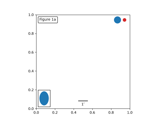
misc/bbox_intersect
==================================
Source
"""
==================================
Identify whether artists intersect
==================================

The lines intersecting the rectangle are colored in red, while the others
are left as blue lines. This example showcases the `.intersects_bbox` function.

"""

import matplotlib.pyplot as plt
import numpy as np

from matplotlib.path import Path
from matplotlib.transforms import Bbox

# Fixing random state for reproducibility
np.random.seed(19680801)


left, bottom, width, height = (-1, -1, 2, 2)
rect = plt.Rectangle((left, bottom), width, height,
                     facecolor="black", alpha=0.1)

fig, ax = plt.subplots()
ax.add_patch(rect)

bbox = Bbox.from_bounds(left, bottom, width, height)

for i in range(12):
    vertices = (np.random.random((2, 2)) - 0.5) * 6.0
    path = Path(vertices)
    if path.intersects_bbox(bbox):
        color = 'r'
    else:
        color = 'b'
    ax.plot(vertices[:, 0], vertices[:, 1], color=color)

plt.show()
misc/contour_manual
==============
Source
"""
==============
Manual Contour
==============

Example of displaying your own contour lines and polygons using ContourSet.
"""

import matplotlib.pyplot as plt

from matplotlib.contour import ContourSet
from matplotlib.path import Path

# %%
# Contour lines for each level are a list/tuple of polygons.
lines0 = [[[0, 0], [0, 4]]]
lines1 = [[[2, 0], [1, 2], [1, 3]]]
lines2 = [[[3, 0], [3, 2]], [[3, 3], [3, 4]]]  # Note two lines.

# %%
# Filled contours between two levels are also a list/tuple of polygons.
# Points can be ordered clockwise or anticlockwise.
filled01 = [[[0, 0], [0, 4], [1, 3], [1, 2], [2, 0]]]
filled12 = [[[2, 0], [3, 0], [3, 2], [1, 3], [1, 2]],   # Note two polygons.
            [[1, 4], [3, 4], [3, 3]]]

# %%

fig, ax = plt.subplots()

# Filled contours using filled=True.
cs = ContourSet(ax, [0, 1, 2], [filled01, filled12], filled=True, cmap="bone")
cbar = fig.colorbar(cs)

# Contour lines (non-filled).
lines = ContourSet(
    ax, [0, 1, 2], [lines0, lines1, lines2], cmap="cool", linewidths=3)
cbar.add_lines(lines)

ax.set(xlim=(-0.5, 3.5), ylim=(-0.5, 4.5),
       title='User-specified contours')

# %%
# Multiple filled contour lines can be specified in a single list of polygon
# vertices along with a list of vertex kinds (code types) as described in the
# Path class.  This is particularly useful for polygons with holes.

fig, ax = plt.subplots()
filled01 = [[[0, 0], [3, 0], [3, 3], [0, 3], [1, 1], [1, 2], [2, 2], [2, 1]]]
M = Path.MOVETO
L = Path.LINETO
kinds01 = [[M, L, L, L, M, L, L, L]]
cs = ContourSet(ax, [0, 1], [filled01], [kinds01], filled=True)
cbar = fig.colorbar(cs)

ax.set(xlim=(-0.5, 3.5), ylim=(-0.5, 3.5),
       title='User specified filled contours with holes')

plt.show()
NotImplementedError: user-specified contour paths are not supported yet
misc/coords_report
=============
Source
"""
=============
Coords Report
=============

Override the default reporting of coords as the mouse moves over the Axes
in an interactive backend.
"""

import matplotlib.pyplot as plt
import numpy as np


def millions(x):
    return '$%1.1fM' % (x * 1e-6)


# Fixing random state for reproducibility
np.random.seed(19680801)

x = np.random.rand(20)
y = 1e7 * np.random.rand(20)

fig, ax = plt.subplots()
ax.fmt_ydata = millions
plt.plot(x, y, 'o')

plt.show()
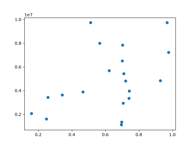
misc/custom_projection
=================
Source
"""
=================
Custom projection
=================

Showcase Hammer projection by alleviating many features of Matplotlib.
"""

import numpy as np

import matplotlib
from matplotlib.axes import Axes
import matplotlib.axis as maxis
from matplotlib.patches import Circle
from matplotlib.path import Path
from matplotlib.projections import register_projection
import matplotlib.spines as mspines
from matplotlib.ticker import FixedLocator, Formatter, NullLocator
from matplotlib.transforms import Affine2D, BboxTransformTo, Transform

rcParams = matplotlib.rcParams

# This example projection class is rather long, but it is designed to
# illustrate many features, not all of which will be used every time.
# It is also common to factor out a lot of these methods into common
# code used by a number of projections with similar characteristics
# (see geo.py).


class GeoAxes(Axes):
    """
    An abstract base class for geographic projections
    """
    class ThetaFormatter(Formatter):
        """
        Used to format the theta tick labels.  Converts the native
        unit of radians into degrees and adds a degree symbol.
        """
        def __init__(self, round_to=1.0):
            self._round_to = round_to

        def __call__(self, x, pos=None):
            degrees = round(np.rad2deg(x) / self._round_to) * self._round_to
            return f"{degrees:0.0f}\N{DEGREE SIGN}"

    RESOLUTION = 75

    def _init_axis(self):
        self.xaxis = maxis.XAxis(self)
        self.yaxis = maxis.YAxis(self)
        # Do not register xaxis or yaxis with spines -- as done in
        # Axes._init_axis() -- until GeoAxes.xaxis.clear() works.
        # self.spines['geo'].register_axis(self.yaxis)

    def clear(self):
        # docstring inherited
        super().clear()

        self.set_longitude_grid(30)
        self.set_latitude_grid(15)
        self.set_longitude_grid_ends(75)
        self.xaxis.set_minor_locator(NullLocator())
        self.yaxis.set_minor_locator(NullLocator())
        self.xaxis.set_ticks_position('none')
        self.yaxis.set_ticks_position('none')
        self.yaxis.set_tick_params(label1On=True)
        # Why do we need to turn on yaxis tick labels, but
        # xaxis tick labels are already on?

        self.grid(rcParams['axes.grid'])

        Axes.set_xlim(self, -np.pi, np.pi)
        Axes.set_ylim(self, -np.pi / 2.0, np.pi / 2.0)

    def _set_lim_and_transforms(self):
        # A (possibly non-linear) projection on the (already scaled) data

        # There are three important coordinate spaces going on here:
        #
        # 1. Data space: The space of the data itself
        #
        # 2. Axes space: The unit rectangle (0, 0) to (1, 1)
        #    covering the entire plot area.
        #
        # 3. Display space: The coordinates of the resulting image,
        #    often in pixels or dpi/inch.

        # This function makes heavy use of the Transform classes in
        # ``lib/matplotlib/transforms.py.`` For more information, see
        # the inline documentation there.

        # The goal of the first two transformations is to get from the
        # data space (in this case longitude and latitude) to Axes
        # space.  It is separated into a non-affine and affine part so
        # that the non-affine part does not have to be recomputed when
        # a simple affine change to the figure has been made (such as
        # resizing the window or changing the dpi).

        # 1) The core transformation from data space into
        # rectilinear space defined in the HammerTransform class.
        self.transProjection = self._get_core_transform(self.RESOLUTION)

        # 2) The above has an output range that is not in the unit
        # rectangle, so scale and translate it so it fits correctly
        # within the Axes.  The peculiar calculations of xscale and
        # yscale are specific to an Aitoff-Hammer projection, so don't
        # worry about them too much.
        self.transAffine = self._get_affine_transform()

        # 3) This is the transformation from Axes space to display
        # space.
        self.transAxes = BboxTransformTo(self.bbox)

        # Now put these 3 transforms together -- from data all the way
        # to display coordinates.  Using the '+' operator, these
        # transforms will be applied "in order".  The transforms are
        # automatically simplified, if possible, by the underlying
        # transformation framework.
        self.transData = \
            self.transProjection + \
            self.transAffine + \
            self.transAxes

        # The main data transformation is set up.  Now deal with
        # gridlines and tick labels.

        # Longitude gridlines and ticklabels.  The input to these
        # transforms are in display space in x and Axes space in y.
        # Therefore, the input values will be in range (-xmin, 0),
        # (xmax, 1).  The goal of these transforms is to go from that
        # space to display space.  The tick labels will be offset 4
        # pixels from the equator.
        self._xaxis_pretransform = \
            Affine2D() \
            .scale(1.0, self._longitude_cap * 2.0) \
            .translate(0.0, -self._longitude_cap)
        self._xaxis_transform = \
            self._xaxis_pretransform + \
            self.transData
        self._xaxis_text1_transform = \
            Affine2D().scale(1.0, 0.0) + \
            self.transData + \
            Affine2D().translate(0.0, 4.0)
        self._xaxis_text2_transform = \
            Affine2D().scale(1.0, 0.0) + \
            self.transData + \
            Affine2D().translate(0.0, -4.0)

        # Now set up the transforms for the latitude ticks.  The input to
        # these transforms are in Axes space in x and display space in
        # y.  Therefore, the input values will be in range (0, -ymin),
        # (1, ymax).  The goal of these transforms is to go from that
        # space to display space.  The tick labels will be offset 4
        # pixels from the edge of the Axes ellipse.
        yaxis_stretch = Affine2D().scale(np.pi*2, 1).translate(-np.pi, 0)
        yaxis_space = Affine2D().scale(1.0, 1.1)
        self._yaxis_transform = \
            yaxis_stretch + \
            self.transData
        yaxis_text_base = \
            yaxis_stretch + \
            self.transProjection + \
            (yaxis_space +
             self.transAffine +
             self.transAxes)
        self._yaxis_text1_transform = \
            yaxis_text_base + \
            Affine2D().translate(-8.0, 0.0)
        self._yaxis_text2_transform = \
            yaxis_text_base + \
            Affine2D().translate(8.0, 0.0)

    def _get_affine_transform(self):
        transform = self._get_core_transform(1)
        xscale, _ = transform.transform((np.pi, 0))
        _, yscale = transform.transform((0, np.pi/2))
        return Affine2D() \
            .scale(0.5 / xscale, 0.5 / yscale) \
            .translate(0.5, 0.5)

    def get_xaxis_transform(self, which='grid'):
        """
        Override this method to provide a transformation for the
        x-axis tick labels.

        Returns a tuple of the form (transform, valign, halign)
        """
        if which not in ['tick1', 'tick2', 'grid']:
            raise ValueError(
                "'which' must be one of 'tick1', 'tick2', or 'grid'")
        return self._xaxis_transform

    def get_xaxis_text1_transform(self, pad):
        return self._xaxis_text1_transform, 'bottom', 'center'

    def get_xaxis_text2_transform(self, pad):
        """
        Override this method to provide a transformation for the
        secondary x-axis tick labels.

        Returns a tuple of the form (transform, valign, halign)
        """
        return self._xaxis_text2_transform, 'top', 'center'

    def get_yaxis_transform(self, which='grid'):
        """
        Override this method to provide a transformation for the
        y-axis grid and ticks.
        """
        if which not in ['tick1', 'tick2', 'grid']:
            raise ValueError(
                "'which' must be one of 'tick1', 'tick2', or 'grid'")
        return self._yaxis_transform

    def get_yaxis_text1_transform(self, pad):
        """
        Override this method to provide a transformation for the
        y-axis tick labels.

        Returns a tuple of the form (transform, valign, halign)
        """
        return self._yaxis_text1_transform, 'center', 'right'

    def get_yaxis_text2_transform(self, pad):
        """
        Override this method to provide a transformation for the
        secondary y-axis tick labels.

        Returns a tuple of the form (transform, valign, halign)
        """
        return self._yaxis_text2_transform, 'center', 'left'

    def _gen_axes_patch(self):
        """
        Override this method to define the shape that is used for the
        background of the plot.  It should be a subclass of Patch.

        In this case, it is a Circle (that may be warped by the Axes
        transform into an ellipse).  Any data and gridlines will be
        clipped to this shape.
        """
        return Circle((0.5, 0.5), 0.5)

    def _gen_axes_spines(self):
        return {'geo': mspines.Spine.circular_spine(self, (0.5, 0.5), 0.5)}

    def set_yscale(self, *args, **kwargs):
        if args[0] != 'linear':
            raise NotImplementedError

    # Prevent the user from applying scales to one or both of the
    # axes.  In this particular case, scaling the axes wouldn't make
    # sense, so we don't allow it.
    set_xscale = set_yscale

    # Prevent the user from changing the axes limits.  In our case, we
    # want to display the whole sphere all the time, so we override
    # set_xlim and set_ylim to ignore any input.  This also applies to
    # interactive panning and zooming in the GUI interfaces.
    def set_xlim(self, *args, **kwargs):
        raise TypeError("Changing axes limits of a geographic projection is "
                        "not supported.  Please consider using Cartopy.")

    set_ylim = set_xlim

    def format_coord(self, lon, lat):
        """
        Override this method to change how the values are displayed in
        the status bar.

        In this case, we want them to be displayed in degrees N/S/E/W.
        """
        lon, lat = np.rad2deg([lon, lat])
        ns = 'N' if lat >= 0.0 else 'S'
        ew = 'E' if lon >= 0.0 else 'W'
        return ('%f\N{DEGREE SIGN}%s, %f\N{DEGREE SIGN}%s'
                % (abs(lat), ns, abs(lon), ew))

    def set_longitude_grid(self, degrees):
        """
        Set the number of degrees between each longitude grid.

        This is an example method that is specific to this projection
        class -- it provides a more convenient interface to set the
        ticking than set_xticks would.
        """
        # Skip -180 and 180, which are the fixed limits.
        grid = np.arange(-180 + degrees, 180, degrees)
        self.xaxis.set_major_locator(FixedLocator(np.deg2rad(grid)))
        self.xaxis.set_major_formatter(self.ThetaFormatter(degrees))

    def set_latitude_grid(self, degrees):
        """
        Set the number of degrees between each longitude grid.

        This is an example method that is specific to this projection
        class -- it provides a more convenient interface than
        set_yticks would.
        """
        # Skip -90 and 90, which are the fixed limits.
        grid = np.arange(-90 + degrees, 90, degrees)
        self.yaxis.set_major_locator(FixedLocator(np.deg2rad(grid)))
        self.yaxis.set_major_formatter(self.ThetaFormatter(degrees))

    def set_longitude_grid_ends(self, degrees):
        """
        Set the latitude(s) at which to stop drawing the longitude grids.

        Often, in geographic projections, you wouldn't want to draw
        longitude gridlines near the poles.  This allows the user to
        specify the degree at which to stop drawing longitude grids.

        This is an example method that is specific to this projection
        class -- it provides an interface to something that has no
        analogy in the base Axes class.
        """
        self._longitude_cap = np.deg2rad(degrees)
        self._xaxis_pretransform \
            .clear() \
            .scale(1.0, self._longitude_cap * 2.0) \
            .translate(0.0, -self._longitude_cap)

    def get_data_ratio(self):
        """
        Return the aspect ratio of the data itself.

        This method should be overridden by any Axes that have a
        fixed data ratio.
        """
        return 1.0

    # Interactive panning and zooming is not supported with this projection,
    # so we override all of the following methods to disable it.
    def can_zoom(self):
        """
        Return whether this Axes supports the zoom box button functionality.

        This Axes object does not support interactive zoom box.
        """
        return False

    def can_pan(self):
        """
        Return whether this Axes supports the pan/zoom button functionality.

        This Axes object does not support interactive pan/zoom.
        """
        return False

    def start_pan(self, x, y, button):
        pass

    def end_pan(self):
        pass

    def drag_pan(self, button, key, x, y):
        pass


class HammerAxes(GeoAxes):
    """
    A custom class for the Aitoff-Hammer projection, an equal-area map
    projection.

    https://en.wikipedia.org/wiki/Hammer_projection
    """

    # The projection must specify a name. This will be used by the
    # user to select the projection,
    # i.e. ``subplot(projection='custom_hammer')``.
    name = 'custom_hammer'

    class HammerTransform(Transform):
        """The base Hammer transform."""
        input_dims = output_dims = 2

        def __init__(self, resolution):
            """
            Create a new Hammer transform.  Resolution is the number of steps
            to interpolate between each input line segment to approximate its
            path in curved Hammer space.
            """
            Transform.__init__(self)
            self._resolution = resolution

        def transform_non_affine(self, ll):
            longitude, latitude = ll.T

            # Pre-compute some values
            half_long = longitude / 2
            cos_latitude = np.cos(latitude)
            sqrt2 = np.sqrt(2)

            alpha = np.sqrt(1 + cos_latitude * np.cos(half_long))
            x = (2 * sqrt2) * (cos_latitude * np.sin(half_long)) / alpha
            y = (sqrt2 * np.sin(latitude)) / alpha
            return np.column_stack([x, y])

        def transform_path_non_affine(self, path):
            # vertices = path.vertices
            ipath = path.interpolated(self._resolution)
            return Path(self.transform(ipath.vertices), ipath.codes)

        def inverted(self):
            return HammerAxes.InvertedHammerTransform(self._resolution)

    class InvertedHammerTransform(Transform):
        input_dims = output_dims = 2

        def __init__(self, resolution):
            Transform.__init__(self)
            self._resolution = resolution

        def transform_non_affine(self, xy):
            x, y = xy.T
            z = np.sqrt(1 - (x / 4) ** 2 - (y / 2) ** 2)
            longitude = 2 * np.arctan((z * x) / (2 * (2 * z ** 2 - 1)))
            latitude = np.arcsin(y*z)
            return np.column_stack([longitude, latitude])

        def inverted(self):
            return HammerAxes.HammerTransform(self._resolution)

    def __init__(self, *args, **kwargs):
        self._longitude_cap = np.pi / 2.0
        super().__init__(*args, **kwargs)
        self.set_aspect(0.5, adjustable='box', anchor='C')
        self.clear()

    def _get_core_transform(self, resolution):
        return self.HammerTransform(resolution)


# Now register the projection with Matplotlib so the user can select it.
register_projection(HammerAxes)


if __name__ == '__main__':
    import matplotlib.pyplot as plt

    # Now make a simple example using the custom projection.
    fig, ax = plt.subplots(subplot_kw={'projection': 'custom_hammer'})
    ax.plot([-1, 1, 1], [-1, -1, 1], "o-")
    ax.grid()

    plt.show()
misc/customize_rc
============
Source
"""
============
Customize Rc
============

I'm not trying to make a good-looking figure here, but just to show
some examples of customizing `.rcParams` on the fly.

If you like to work interactively, and need to create different sets
of defaults for figures (e.g., one set of defaults for publication, one
set for interactive exploration), you may want to define some
functions in a custom module that set the defaults, e.g.,::

    def set_pub():
        rcParams.update({
            "font.weight": "bold",  # bold fonts
            "tick.labelsize": 15,   # large tick labels
            "lines.linewidth": 1,   # thick lines
            "lines.color": "k",     # black lines
            "grid.color": "0.5",    # gray gridlines
            "grid.linestyle": "-",  # solid gridlines
            "grid.linewidth": 0.5,  # thin gridlines
            "savefig.dpi": 300,     # higher resolution output.
        })

Then as you are working interactively, you just need to do::

    >>> set_pub()
    >>> plot([1, 2, 3])
    >>> savefig('myfig')
    >>> rcdefaults()  # restore the defaults
"""

import matplotlib.pyplot as plt

plt.subplot(311)
plt.plot([1, 2, 3])

# the axes attributes need to be set before the call to subplot
plt.rcParams.update({
    "font.weight": "bold",
    "xtick.major.size": 5,
    "xtick.major.pad": 7,
    "xtick.labelsize": 15,
    "grid.color": "0.5",
    "grid.linestyle": "-",
    "grid.linewidth": 5,
    "lines.linewidth": 2,
    "lines.color": "g",
})
plt.subplot(312)
plt.plot([1, 2, 3])
plt.grid(True)

plt.rcdefaults()
plt.subplot(313)
plt.plot([1, 2, 3])
plt.grid(True)
plt.show()
misc/demo_agg_filter
==========
Source
"""
==========
AGG filter
==========

Most pixel-based backends in Matplotlib use `Anti-Grain Geometry (AGG)`_ for
rendering. You can modify the rendering of Artists by applying a filter via
`.Artist.set_agg_filter`.

.. _Anti-Grain Geometry (AGG): http://agg.sourceforge.net/antigrain.com
"""

import matplotlib.pyplot as plt
import numpy as np

from matplotlib.artist import Artist
from matplotlib.colors import LightSource
import matplotlib.transforms as mtransforms


def smooth1d(x, window_len):
    # copied from https://scipy-cookbook.readthedocs.io/items/SignalSmooth.html
    s = np.r_[2*x[0] - x[window_len:1:-1], x, 2*x[-1] - x[-1:-window_len:-1]]
    w = np.hanning(window_len)
    y = np.convolve(w/w.sum(), s, mode='same')
    return y[window_len-1:-window_len+1]


def smooth2d(A, sigma=3):
    window_len = max(int(sigma), 3) * 2 + 1
    A = np.apply_along_axis(smooth1d, 0, A, window_len)
    A = np.apply_along_axis(smooth1d, 1, A, window_len)
    return A


class BaseFilter:

    def get_pad(self, dpi):
        return 0

    def process_image(self, padded_src, dpi):
        raise NotImplementedError("Should be overridden by subclasses")

    def __call__(self, im, dpi):
        pad = self.get_pad(dpi)
        padded_src = np.pad(im, [(pad, pad), (pad, pad), (0, 0)], "constant")
        tgt_image = self.process_image(padded_src, dpi)
        return tgt_image, -pad, -pad


class OffsetFilter(BaseFilter):

    def __init__(self, offsets=(0, 0)):
        self.offsets = offsets

    def get_pad(self, dpi):
        return int(max(self.offsets) / 72 * dpi)

    def process_image(self, padded_src, dpi):
        ox, oy = self.offsets
        a1 = np.roll(padded_src, int(ox / 72 * dpi), axis=1)
        a2 = np.roll(a1, -int(oy / 72 * dpi), axis=0)
        return a2


class GaussianFilter(BaseFilter):
    """Simple Gaussian filter."""

    def __init__(self, sigma, alpha=0.5, color=(0, 0, 0)):
        self.sigma = sigma
        self.alpha = alpha
        self.color = color

    def get_pad(self, dpi):
        return int(self.sigma*3 / 72 * dpi)

    def process_image(self, padded_src, dpi):
        tgt_image = np.empty_like(padded_src)
        tgt_image[:, :, :3] = self.color
        tgt_image[:, :, 3] = smooth2d(padded_src[:, :, 3] * self.alpha,
                                      self.sigma / 72 * dpi)
        return tgt_image


class DropShadowFilter(BaseFilter):

    def __init__(self, sigma, alpha=0.3, color=(0, 0, 0), offsets=(0, 0)):
        self.gauss_filter = GaussianFilter(sigma, alpha, color)
        self.offset_filter = OffsetFilter(offsets)

    def get_pad(self, dpi):
        return max(self.gauss_filter.get_pad(dpi),
                   self.offset_filter.get_pad(dpi))

    def process_image(self, padded_src, dpi):
        t1 = self.gauss_filter.process_image(padded_src, dpi)
        t2 = self.offset_filter.process_image(t1, dpi)
        return t2


class LightFilter(BaseFilter):
    """Apply LightSource filter"""

    def __init__(self, sigma, fraction=1):
        """
        Parameters
        ----------
        sigma : float
            sigma for gaussian filter
        fraction: number, default: 1
            Increases or decreases the contrast of the hillshade.
            See `matplotlib.colors.LightSource`

        """
        self.gauss_filter = GaussianFilter(sigma, alpha=1)
        self.light_source = LightSource()
        self.fraction = fraction

    def get_pad(self, dpi):
        return self.gauss_filter.get_pad(dpi)

    def process_image(self, padded_src, dpi):
        t1 = self.gauss_filter.process_image(padded_src, dpi)
        elevation = t1[:, :, 3]
        rgb = padded_src[:, :, :3]
        alpha = padded_src[:, :, 3:]
        rgb2 = self.light_source.shade_rgb(rgb, elevation,
                                           fraction=self.fraction,
                                           blend_mode="overlay")
        return np.concatenate([rgb2, alpha], -1)


class GrowFilter(BaseFilter):
    """Enlarge the area."""

    def __init__(self, pixels, color=(1, 1, 1)):
        self.pixels = pixels
        self.color = color

    def __call__(self, im, dpi):
        alpha = np.pad(im[..., 3], self.pixels, "constant")
        alpha2 = np.clip(smooth2d(alpha, self.pixels / 72 * dpi) * 5, 0, 1)
        new_im = np.empty((*alpha2.shape, 4))
        new_im[:, :, :3] = self.color
        new_im[:, :, 3] = alpha2
        offsetx, offsety = -self.pixels, -self.pixels
        return new_im, offsetx, offsety


class FilteredArtistList(Artist):
    """A simple container to filter multiple artists at once."""

    def __init__(self, artist_list, filter):
        super().__init__()
        self._artist_list = artist_list
        self._filter = filter

    def draw(self, renderer):
        renderer.start_rasterizing()
        renderer.start_filter()
        for a in self._artist_list:
            a.draw(renderer)
        renderer.stop_filter(self._filter)
        renderer.stop_rasterizing()


def filtered_text(ax):
    # mostly copied from contour_demo.py

    # prepare image
    delta = 0.025
    x = np.arange(-3.0, 3.0, delta)
    y = np.arange(-2.0, 2.0, delta)
    X, Y = np.meshgrid(x, y)
    Z1 = np.exp(-X**2 - Y**2)
    Z2 = np.exp(-(X - 1)**2 - (Y - 1)**2)
    Z = (Z1 - Z2) * 2

    # draw
    ax.imshow(Z, interpolation='bilinear', origin='lower',
              cmap="gray", extent=(-3, 3, -2, 2), aspect='auto')
    levels = np.arange(-1.2, 1.6, 0.2)
    CS = ax.contour(Z, levels,
                    origin='lower',
                    linewidths=2,
                    extent=(-3, 3, -2, 2))

    # contour label
    cl = ax.clabel(CS, levels[1::2],  # label every second level
                   fmt='%1.1f',
                   fontsize=11)

    # change clabel color to black
    from matplotlib.patheffects import Normal
    for t in cl:
        t.set_color("k")
        # to force TextPath (i.e., same font in all backends)
        t.set_path_effects([Normal()])

    # Add white glows to improve visibility of labels.
    white_glows = FilteredArtistList(cl, GrowFilter(3))
    ax.add_artist(white_glows)
    white_glows.set_zorder(cl[0].get_zorder() - 0.1)

    ax.xaxis.set_visible(False)
    ax.yaxis.set_visible(False)


def drop_shadow_line(ax):
    # copied from examples/misc/svg_filter_line.py

    # draw lines
    l1, = ax.plot([0.1, 0.5, 0.9], [0.1, 0.9, 0.5], "bo-")
    l2, = ax.plot([0.1, 0.5, 0.9], [0.5, 0.2, 0.7], "ro-")

    gauss = DropShadowFilter(4)

    for l in [l1, l2]:

        # draw shadows with same lines with slight offset.
        xx = l.get_xdata()
        yy = l.get_ydata()
        shadow, = ax.plot(xx, yy)
        shadow.update_from(l)

        # offset transform
        transform = mtransforms.offset_copy(l.get_transform(), ax.figure,
                                            x=4.0, y=-6.0, units='points')
        shadow.set_transform(transform)

        # adjust zorder of the shadow lines so that it is drawn below the
        # original lines
        shadow.set_zorder(l.get_zorder() - 0.5)
        shadow.set_agg_filter(gauss)
        shadow.set_rasterized(True)  # to support mixed-mode renderers

    ax.set_xlim(0., 1.)
    ax.set_ylim(0., 1.)

    ax.xaxis.set_visible(False)
    ax.yaxis.set_visible(False)


def drop_shadow_patches(ax):
    # Copied from barchart_demo.py
    N = 5
    group1_means = [20, 35, 30, 35, 27]

    ind = np.arange(N)  # the x locations for the groups
    width = 0.35  # the width of the bars

    rects1 = ax.bar(ind, group1_means, width, color='r', ec="w", lw=2)

    group2_means = [25, 32, 34, 20, 25]
    rects2 = ax.bar(ind + width + 0.1, group2_means, width,
                    color='y', ec="w", lw=2)

    drop = DropShadowFilter(5, offsets=(1, 1))
    shadow = FilteredArtistList(rects1 + rects2, drop)
    ax.add_artist(shadow)
    shadow.set_zorder(rects1[0].get_zorder() - 0.1)

    ax.set_ylim(0, 40)

    ax.xaxis.set_visible(False)
    ax.yaxis.set_visible(False)


def light_filter_pie(ax):
    fracs = [15, 30, 45, 10]
    explode = (0.1, 0.2, 0.1, 0.1)
    pie = ax.pie(fracs, explode=explode)

    light_filter = LightFilter(9)
    for p in pie.wedges:
        p.set_agg_filter(light_filter)
        p.set_rasterized(True)  # to support mixed-mode renderers
        p.set(ec="none",
              lw=2)

    gauss = DropShadowFilter(9, offsets=(3, -4), alpha=0.7)
    shadow = FilteredArtistList(pie.wedges, gauss)
    ax.add_artist(shadow)
    shadow.set_zorder(pie.wedges[0].get_zorder() - 0.1)


if __name__ == "__main__":

    fix, axs = plt.subplots(2, 2)

    filtered_text(axs[0, 0])
    drop_shadow_line(axs[0, 1])
    drop_shadow_patches(axs[1, 0])
    light_filter_pie(axs[1, 1])
    axs[1, 1].set_frame_on(True)

    plt.show()
misc/demo_ribbon_box
==========
Source
"""
==========
Ribbon box
==========

"""

from PIL import Image

import matplotlib.pyplot as plt
import numpy as np

from matplotlib import cbook
from matplotlib import colors as mcolors
from matplotlib.image import AxesImage
from matplotlib.transforms import Bbox, BboxTransformTo, TransformedBbox


class RibbonBox:

    # Image.open reads this image as 8-bit; divide by 255 to convert to 0-1.
    original_image = np.asarray(Image.open(
        cbook.get_sample_data("Minduka_Present_Blue_Pack.png"))) / 255
    cut_location = 70
    b_and_h = original_image[:, :, 2:3]
    color = original_image[:, :, 2:3] - original_image[:, :, 0:1]
    alpha = original_image[:, :, 3:4]
    nx = original_image.shape[1]

    def __init__(self, color):
        rgb = mcolors.to_rgb(color)
        self.im = np.dstack(
            [self.b_and_h - self.color * (1 - np.array(rgb)), self.alpha])

    def get_stretched_image(self, stretch_factor):
        stretch_factor = max(stretch_factor, 1)
        ny, nx, nch = self.im.shape
        ny2 = int(ny*stretch_factor)
        return np.vstack(
            [self.im[:self.cut_location],
             np.broadcast_to(
                 self.im[self.cut_location], (ny2 - ny, nx, nch)),
             self.im[self.cut_location:]])


class RibbonBoxImage(AxesImage):
    zorder = 1

    def __init__(self, ax, bbox, color, *, extent=(0, 1, 0, 1), **kwargs):
        super().__init__(ax, extent=extent, **kwargs)
        self._bbox = bbox
        self._ribbonbox = RibbonBox(color)
        self.set_transform(BboxTransformTo(bbox))

    def draw(self, renderer):
        stretch_factor = self._bbox.height / self._bbox.width

        ny = int(stretch_factor*self._ribbonbox.nx)
        if self.get_array() is None or self.get_array().shape[0] != ny:
            arr = self._ribbonbox.get_stretched_image(stretch_factor)
            self.set_array(arr)

        super().draw(renderer)


def main():
    fig, ax = plt.subplots()

    years = np.arange(2004, 2009)
    heights = [7900, 8100, 7900, 6900, 2800]
    box_colors = [
        (0.8, 0.2, 0.2),
        (0.2, 0.8, 0.2),
        (0.2, 0.2, 0.8),
        (0.7, 0.5, 0.8),
        (0.3, 0.8, 0.7),
    ]

    for year, h, bc in zip(years, heights, box_colors):
        bbox0 = Bbox.from_extents(year - 0.4, 0., year + 0.4, h)
        bbox = TransformedBbox(bbox0, ax.transData)
        ax.add_artist(RibbonBoxImage(ax, bbox, bc, interpolation="bicubic"))
        ax.annotate(str(h), (year, h), va="bottom", ha="center")

    ax.set_xlim(years[0] - 0.5, years[-1] + 0.5)
    ax.set_ylim(0, 10000)

    background_gradient = np.zeros((2, 2, 4))
    background_gradient[:, :, :3] = [1, 1, 0]
    background_gradient[:, :, 3] = [[0.1, 0.3], [0.3, 0.5]]  # alpha channel
    ax.imshow(background_gradient, interpolation="bicubic", zorder=0.1,
              extent=(0, 1, 0, 1), transform=ax.transAxes)

    plt.show()


main()
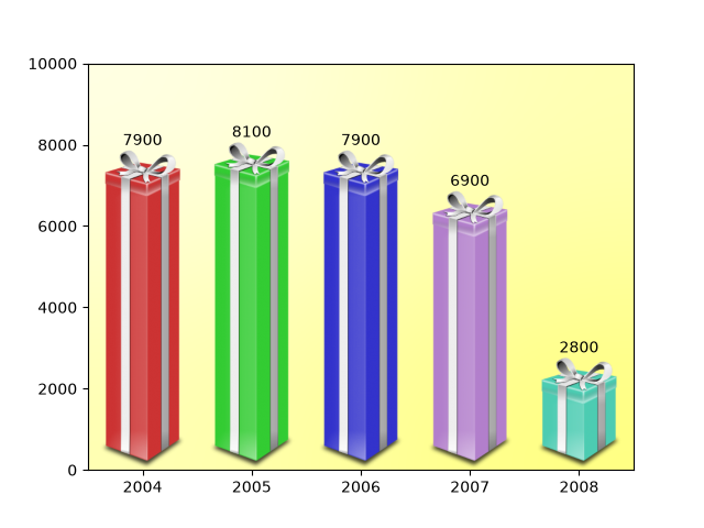
misc/fig_x
==============================
Source
"""
==============================
Add lines directly to a figure
==============================

You can add artists such as a `.Line2D` directly to a figure. This is
typically useful for visual structuring.

.. redirect-from:: /gallery/pyplots/fig_x
"""

import matplotlib.pyplot as plt

import matplotlib.lines as lines

fig, axs = plt.subplots(2, 2, gridspec_kw={'hspace': 0.4, 'wspace': 0.4})
fig.add_artist(lines.Line2D([0, 1], [0.47, 0.47], linewidth=3))
fig.add_artist(lines.Line2D([0.5, 0.5], [1, 0], linewidth=3))
plt.show()

# %%
#
# .. admonition:: References
#
#    The use of the following functions, methods, classes and modules is shown
#    in this example:
#
#    - `matplotlib.pyplot.figure`
#    - `matplotlib.lines`
#    - `matplotlib.lines.Line2D`
misc/fill_spiral
===========
Source
"""
===========
Fill spiral
===========

"""
import matplotlib.pyplot as plt
import numpy as np

theta = np.arange(0, 8*np.pi, 0.1)
a = 1
b = .2

for dt in np.arange(0, 2*np.pi, np.pi/2.0):

    x = a*np.cos(theta + dt)*np.exp(b*theta)
    y = a*np.sin(theta + dt)*np.exp(b*theta)

    dt = dt + np.pi/4.0

    x2 = a*np.cos(theta + dt)*np.exp(b*theta)
    y2 = a*np.sin(theta + dt)*np.exp(b*theta)

    xf = np.concatenate((x, x2[::-1]))
    yf = np.concatenate((y, y2[::-1]))

    p1 = plt.fill(xf, yf)

plt.show()
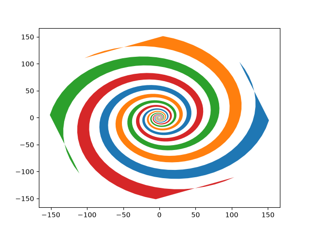
misc/findobj_demo
============
Source
"""
============
Findobj Demo
============

Recursively find all objects that match some criteria
"""
import matplotlib.pyplot as plt
import numpy as np

import matplotlib.text as text

a = np.arange(0, 3, .02)
b = np.arange(0, 3, .02)
c = np.exp(a)
d = c[::-1]

fig, ax = plt.subplots()
plt.plot(a, c, 'k--', a, d, 'k:', a, c + d, 'k')
plt.legend(('Model length', 'Data length', 'Total message length'),
           loc='upper center', shadow=True)
plt.ylim([-1, 20])
plt.grid(False)
plt.xlabel('Model complexity --->')
plt.ylabel('Message length --->')
plt.title('Minimum Message Length')


# match on arbitrary function
def myfunc(x):
    return hasattr(x, 'set_color') and not hasattr(x, 'set_facecolor')


for o in fig.findobj(myfunc):
    o.set_color('blue')

# match on class instances
for o in fig.findobj(text.Text):
    o.set_fontstyle('italic')


plt.show()
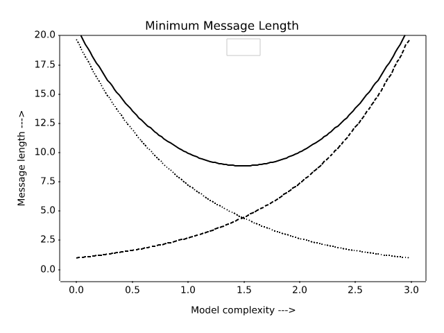
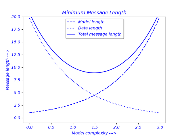
misc/font_indexing
=============
Source
"""
=============
Font indexing
=============

This example shows how the font tables relate to one another.
"""

import os

import matplotlib
from matplotlib.ft2font import FT2Font, Kerning

font = FT2Font(
    os.path.join(matplotlib.get_data_path(), 'fonts/ttf/DejaVuSans.ttf'))
font.set_charmap(0)

codes = font.get_charmap().items()

# make a charname to charcode and glyphind dictionary
coded = {}
glyphd = {}
for ccode, glyphind in codes:
    name = font.get_glyph_name(glyphind)
    coded[name] = ccode
    glyphd[name] = glyphind
    # print(glyphind, ccode, hex(int(ccode)), name)

code = coded['A']
glyph = font.load_char(code)
print(glyph.bbox)
print(glyphd['A'], glyphd['V'], coded['A'], coded['V'])
print('AV', font.get_kerning(glyphd['A'], glyphd['V'], Kerning.DEFAULT))
print('AV', font.get_kerning(glyphd['A'], glyphd['V'], Kerning.UNFITTED))
print('AV', font.get_kerning(glyphd['A'], glyphd['V'], Kerning.UNSCALED))
print('AT', font.get_kerning(glyphd['A'], glyphd['T'], Kerning.UNSCALED))
AttributeError: 'FT2Font' object has no attribute 'set_charmap'
no figure saved
misc/ftface_props
===============
Source
"""
===============
Font properties
===============

This example lists the attributes of an `.FT2Font` object, which describe
global font properties.  For individual character metrics, use the `.Glyph`
object, as returned by `.load_char`.
"""

import os

import matplotlib
import matplotlib.ft2font as ft

font = ft.FT2Font(
    # Use a font shipped with Matplotlib.
    os.path.join(matplotlib.get_data_path(),
                 'fonts/ttf/DejaVuSans-Oblique.ttf'))

print('Num instances:  ', font.num_named_instances)  # number of named instances in file
print('Num faces:      ', font.num_faces)            # number of faces in file
print('Num glyphs:     ', font.num_glyphs)           # number of glyphs in the face
print('Family name:    ', font.family_name)          # face family name
print('Style name:     ', font.style_name)           # face style name
print('PS name:        ', font.postscript_name)      # the postscript name
print('Num fixed:      ', font.num_fixed_sizes)      # number of embedded bitmaps

# the following are only available if face.scalable
if font.scalable:
    # the face global bounding box (xmin, ymin, xmax, ymax)
    print('Bbox:               ', font.bbox)
    # number of font units covered by the EM
    print('EM:                 ', font.units_per_EM)
    # the ascender in 26.6 units
    print('Ascender:           ', font.ascender)
    # the descender in 26.6 units
    print('Descender:          ', font.descender)
    # the height in 26.6 units
    print('Height:             ', font.height)
    # maximum horizontal cursor advance
    print('Max adv width:      ', font.max_advance_width)
    # same for vertical layout
    print('Max adv height:     ', font.max_advance_height)
    # vertical position of the underline bar
    print('Underline pos:      ', font.underline_position)
    # vertical thickness of the underline
    print('Underline thickness:', font.underline_thickness)

for flag in ft.StyleFlags:
    name = flag.name.replace('_', ' ').title() + ':'
    print(f"{name:17}", flag in font.style_flags)

for flag in ft.FaceFlags:
    name = flag.name.replace('_', ' ').title() + ':'
    print(f"{name:17}", flag in font.face_flags)
AttributeError: 'FT2Font' object has no attribute 'num_named_instances'
no figure saved
misc/histogram_path
========================================================
Source
"""
========================================================
Building histograms using Rectangles and PolyCollections
========================================================

Using a path patch to draw rectangles.

The technique of using lots of `.Rectangle` instances, or the faster method of
using `.PolyCollection`, were implemented before we had proper paths with
moveto, lineto, closepoly, etc. in Matplotlib.  Now that we have them, we can
draw collections of regularly shaped objects with homogeneous properties more
efficiently with a PathCollection. This example makes a histogram -- it's more
work to set up the vertex arrays at the outset, but it should be much faster
for large numbers of objects.
"""

import matplotlib.pyplot as plt
import numpy as np

import matplotlib.patches as patches
import matplotlib.path as path

np.random.seed(19680801)  # Fixing random state for reproducibility

# histogram our data with numpy
data = np.random.randn(1000)
n, bins = np.histogram(data, 50)

# get the corners of the rectangles for the histogram
left = bins[:-1]
right = bins[1:]
bottom = np.zeros(len(left))
top = bottom + n

# we need a (numrects x numsides x 2) numpy array for the path helper
# function to build a compound path
XY = np.array([[left, left, right, right], [bottom, top, top, bottom]]).T

# get the Path object
barpath = path.Path.make_compound_path_from_polys(XY)

# make a patch out of it, don't add a margin at y=0
patch = patches.PathPatch(barpath)
patch.sticky_edges.y[:] = [0]

fig, ax = plt.subplots()
ax.add_patch(patch)
ax.autoscale_view()
plt.show()

# %%
# Instead of creating a three-dimensional array and using
# `~.path.Path.make_compound_path_from_polys`, we could as well create the
# compound path directly using vertices and codes as shown below

nrects = len(left)
nverts = nrects*(1+3+1)
verts = np.zeros((nverts, 2))
codes = np.ones(nverts, int) * path.Path.LINETO
codes[0::5] = path.Path.MOVETO
codes[4::5] = path.Path.CLOSEPOLY
verts[0::5, 0] = left
verts[0::5, 1] = bottom
verts[1::5, 0] = left
verts[1::5, 1] = top
verts[2::5, 0] = right
verts[2::5, 1] = top
verts[3::5, 0] = right
verts[3::5, 1] = bottom

barpath = path.Path(verts, codes)

# make a patch out of it, don't add a margin at y=0
patch = patches.PathPatch(barpath)
patch.sticky_edges.y[:] = [0]

fig, ax = plt.subplots()
ax.add_patch(patch)
ax.autoscale_view()
plt.show()

# %%
#
# .. admonition:: References
#
#    The use of the following functions, methods, classes and modules is shown
#    in this example:
#
#    - `matplotlib.patches`
#    - `matplotlib.patches.PathPatch`
#    - `matplotlib.path`
#    - `matplotlib.path.Path`
#    - `matplotlib.path.Path.make_compound_path_from_polys`
#    - `matplotlib.axes.Axes.add_patch`
#    - `matplotlib.collections.PathCollection`
#
#    This example shows an alternative to
#
#    - `matplotlib.collections.PolyCollection`
#    - `matplotlib.axes.Axes.hist`
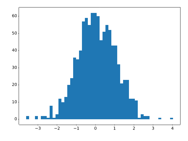
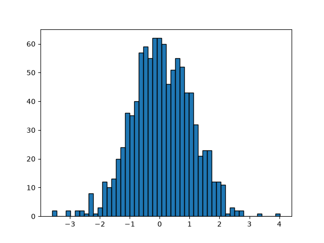
misc/hyperlinks_sgskip
==========
Source
"""
==========
Hyperlinks
==========

This example demonstrates how to set a hyperlinks on various kinds of elements.

This currently only works with the SVG backend.

"""


import matplotlib.pyplot as plt
import numpy as np

# %%

fig = plt.figure()
s = plt.scatter([1, 2, 3], [4, 5, 6])
s.set_urls(['https://www.bbc.com/news', 'https://www.google.com/', None])
fig.savefig('scatter.svg')

# %%
# .. raw:: html
#
#    <object data="../../_static/scatter.svg" type="image/svg+xml"></object>

# %%

fig = plt.figure()
delta = 0.025
x = y = np.arange(-3.0, 3.0, delta)
X, Y = np.meshgrid(x, y)
Z1 = np.exp(-X**2 - Y**2)
Z2 = np.exp(-(X - 1)**2 - (Y - 1)**2)
Z = (Z1 - Z2) * 2

im = plt.imshow(Z, interpolation='bilinear', cmap="gray",
                origin='lower', extent=(-3, 3, -3, 3))

im.set_url('https://www.google.com/')
fig.savefig('image.svg')

# %%
# .. raw:: html
#
#    <object data="../../_static/image.svg" type="image/svg+xml"></object>
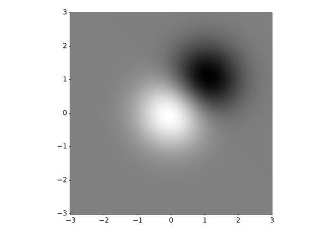
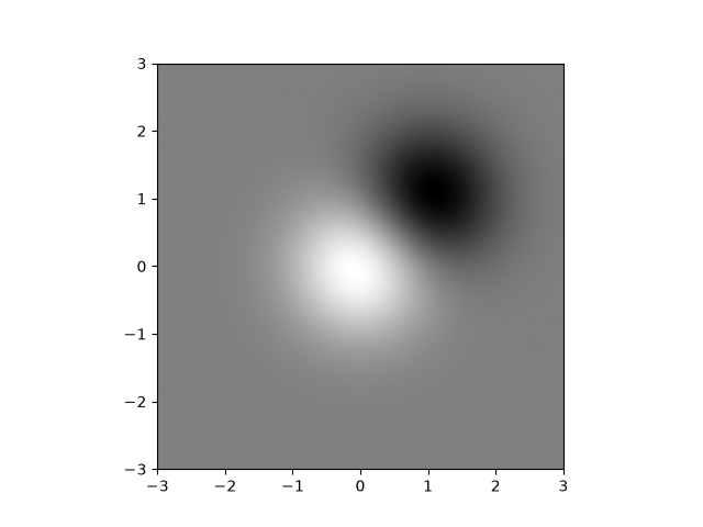
misc/keyword_plotting
======================
Source
"""
======================
Plotting with keywords
======================

Some data structures, like dict, `structured numpy array
<https://numpy.org/doc/stable/user/basics.rec.html#structured-arrays>`_
or `pandas.DataFrame` provide access to labelled data via string index access
``data[key]``.

For these data types, Matplotlib supports passing the whole datastructure via the
``data`` keyword argument, and using the string names as plot function parameters,
where you'd normally pass in your data.
"""

import matplotlib.pyplot as plt
import numpy as np

np.random.seed(19680801)

data = {'a': np.arange(50),
        'c': np.random.randint(0, 50, 50),
        'd': np.random.randn(50)}
data['b'] = data['a'] + 10 * np.random.randn(50)
data['d'] = np.abs(data['d']) * 100

fig, ax = plt.subplots()
ax.scatter('a', 'b', c='c', s='d', data=data)
ax.set(xlabel='entry a', ylabel='entry b')
plt.show()
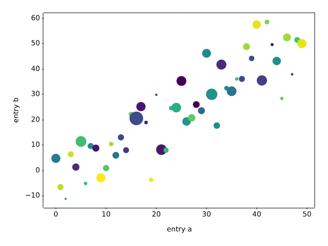
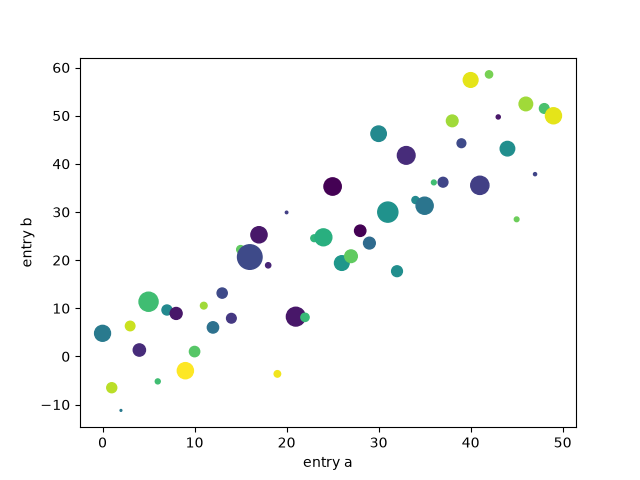
misc/logos2
===============
Source
"""
===============
Matplotlib logo
===============

This example generates the current matplotlib logo.
"""

import matplotlib.pyplot as plt
import numpy as np

import matplotlib.cm as cm
import matplotlib.font_manager
from matplotlib.patches import PathPatch, Rectangle
from matplotlib.text import TextPath
import matplotlib.transforms as mtrans

MPL_BLUE = '#11557c'


def get_font_properties():
    # The original font is Calibri, if that is not installed, we fall back
    # to Carlito, which is metrically equivalent.
    if 'calibri' in matplotlib.font_manager.findfont('Calibri:bold').lower():
        return matplotlib.font_manager.FontProperties(family='Calibri',
                                                      weight='bold')
    # Our website documentation uses Carlito because Calibri is proprietary.
    if 'carlito' in matplotlib.font_manager.findfont('Carlito:bold').lower():
        print('Original font not found. Falling back to Carlito. '
              'The logo text will not be in the correct font.')
        return matplotlib.font_manager.FontProperties(family='Carlito',
                                                      weight='bold')
    print('Original font not found. '
          'The logo text will not be in the correct font.')
    return None


def create_icon_axes(fig, ax_position, lw_bars, lw_grid, lw_border, rgrid):
    """
    Create a polar Axes containing the matplotlib radar plot.

    Parameters
    ----------
    fig : matplotlib.figure.Figure
        The figure to draw into.
    ax_position : (float, float, float, float)
        The position of the created Axes in figure coordinates as
        (x, y, width, height).
    lw_bars : float
        The linewidth of the bars.
    lw_grid : float
        The linewidth of the grid.
    lw_border : float
        The linewidth of the Axes border.
    rgrid : array-like
        Positions of the radial grid.

    Returns
    -------
    ax : matplotlib.axes.Axes
        The created Axes.
    """
    with plt.rc_context({'axes.edgecolor': MPL_BLUE,
                         'axes.linewidth': lw_border}):
        ax = fig.add_axes(ax_position, projection='polar')
        ax.set_axisbelow(True)

        N = 7
        arc = 2. * np.pi
        theta = np.arange(0.0, arc, arc / N)
        radii = np.array([2, 6, 8, 7, 4, 5, 8])
        width = np.pi / 4 * np.array([0.4, 0.4, 0.6, 0.8, 0.2, 0.5, 0.3])
        bars = ax.bar(theta, radii, width=width, bottom=0.0, align='edge',
                      edgecolor='0.3', lw=lw_bars)
        for r, bar in zip(radii, bars):
            color = *cm.jet(r / 10.)[:3], 0.6  # color from jet with alpha=0.6
            bar.set_facecolor(color)

        ax.tick_params(labelbottom=False, labeltop=False,
                       labelleft=False, labelright=False)

        ax.grid(lw=lw_grid, color='0.9')
        ax.set_rmax(9)
        ax.set_yticks(rgrid)

        # the actual visible background - extends a bit beyond the axis
        ax.add_patch(Rectangle((0, 0), arc, 9.58,
                               facecolor='white', zorder=0,
                               clip_on=False, in_layout=False))
        return ax


def create_text_axes(fig, height_px):
    """Create an Axes in *fig* that contains 'matplotlib' as Text."""
    ax = fig.add_axes((0, 0, 1, 1))
    ax.set_aspect("equal")
    ax.set_axis_off()

    path = TextPath((0, 0), "matplotlib", size=height_px * 0.8,
                    prop=get_font_properties())

    angle = 4.25  # degrees
    trans = mtrans.Affine2D().skew_deg(angle, 0)

    patch = PathPatch(path, transform=trans + ax.transData, color=MPL_BLUE,
                      lw=0)
    ax.add_patch(patch)
    ax.autoscale()


def make_logo(height_px, lw_bars, lw_grid, lw_border, rgrid, with_text=False):
    """
    Create a full figure with the Matplotlib logo.

    Parameters
    ----------
    height_px : int
        Height of the figure in pixel.
    lw_bars : float
        The linewidth of the bar border.
    lw_grid : float
        The linewidth of the grid.
    lw_border : float
        The linewidth of icon border.
    rgrid : sequence of float
        The radial grid positions.
    with_text : bool
        Whether to draw only the icon or to include 'matplotlib' as text.
    """
    dpi = 100
    height = height_px / dpi
    figsize = (5 * height, height) if with_text else (height, height)
    fig = plt.figure(figsize=figsize, dpi=dpi)
    fig.patch.set_alpha(0)

    if with_text:
        create_text_axes(fig, height_px)
    ax_pos = (0.535, 0.12, .17, 0.75) if with_text else (0.03, 0.03, .94, .94)
    ax = create_icon_axes(fig, ax_pos, lw_bars, lw_grid, lw_border, rgrid)

    return fig, ax

# %%
# A large logo:

make_logo(height_px=110, lw_bars=0.7, lw_grid=0.5, lw_border=1,
          rgrid=[1, 3, 5, 7])

# %%
# A small 32px logo:

make_logo(height_px=32, lw_bars=0.3, lw_grid=0.3, lw_border=0.3, rgrid=[5])

# %%
# A large logo including text, as used on the matplotlib website.

make_logo(height_px=110, lw_bars=0.7, lw_grid=0.5, lw_border=1,
          rgrid=[1, 3, 5, 7], with_text=True)
plt.show()


misc/multipage_pdf
=============
Source
"""
=============
Multipage PDF
=============

This is a demo of creating a pdf file with several pages,
as well as adding metadata and annotations to pdf files.

"""

import datetime

import matplotlib.pyplot as plt
import numpy as np

from matplotlib.backends.backend_pdf import PdfPages

# sphinx_gallery_thumbnail_path = '_static/multipage_pdf_thumbnail.svg'

# Create the PdfPages object to which we will save the pages:
# The with statement makes sure that the PdfPages object is closed properly at
# the end of the block, even if an Exception occurs.
with PdfPages('multipage_pdf.pdf') as pdf:
    plt.figure(figsize=(3, 3))
    plt.plot(range(7), [3, 1, 4, 1, 5, 9, 2], 'r-o')
    plt.title('Page One')
    pdf.savefig()  # saves the current figure into a pdf page
    plt.close()

    # if LaTeX is not installed or error caught, change to `False`
    plt.rcParams['text.usetex'] = True
    plt.figure(figsize=(8, 6))
    x = np.arange(0, 5, 0.1)
    plt.plot(x, np.sin(x), 'b-')
    plt.title('Page Two')
    pdf.attach_note("plot of sin(x)")  # attach metadata (as pdf note) to page
    pdf.savefig()
    plt.close()

    plt.rcParams['text.usetex'] = False
    fig = plt.figure(figsize=(4, 5))
    plt.plot(x, x ** 2, 'ko')
    plt.title('Page Three')
    pdf.savefig(fig)  # or you can pass a Figure object to pdf.savefig
    plt.close()

    # We can also set the file's metadata via the PdfPages object:
    d = pdf.infodict()
    d['Title'] = 'Multipage PDF Example'
    d['Author'] = 'Jouni K. Sepp\xe4nen'
    d['Subject'] = 'How to create a multipage pdf file and set its metadata'
    d['Keywords'] = 'PdfPages multipage keywords author title subject'
    d['CreationDate'] = datetime.datetime(2009, 11, 13)
    d['ModDate'] = datetime.datetime.today()
NameError: name 'PdfPages' is not defined
RuntimeError: Failed to process string with tex because latex could not be found
misc/multiprocess_sgskip
===============
Source
"""
===============
Multiprocessing
===============

Demo of using multiprocessing for generating data in one process and
plotting in another.

Written by Robert Cimrman
"""

import multiprocessing as mp
import time

import matplotlib.pyplot as plt
import numpy as np

# Fixing random state for reproducibility
np.random.seed(19680801)

# %%
#
# Processing Class
# ================
#
# This class plots data it receives from a pipe.
#


class ProcessPlotter:
    def __init__(self):
        self.x = []
        self.y = []

    def terminate(self):
        plt.close('all')

    def call_back(self):
        while self.pipe.poll():
            command = self.pipe.recv()
            if command is None:
                self.terminate()
                return False
            else:
                self.x.append(command[0])
                self.y.append(command[1])
                self.ax.plot(self.x, self.y, 'ro')
        self.fig.canvas.draw()
        return True

    def __call__(self, pipe):
        print('starting plotter...')

        self.pipe = pipe
        self.fig, self.ax = plt.subplots()
        timer = self.fig.canvas.new_timer(interval=1000)
        timer.add_callback(self.call_back)
        timer.start()

        print('...done')
        plt.show()

# %%
#
# Plotting class
# ==============
#
# This class uses multiprocessing to spawn a process to run code from the
# class above. When initialized, it creates a pipe and an instance of
# ``ProcessPlotter`` which will be run in a separate process.
#
# When run from the command line, the parent process sends data to the spawned
# process which is then plotted via the callback function specified in
# ``ProcessPlotter:__call__``.
#


class NBPlot:
    def __init__(self):
        self.plot_pipe, plotter_pipe = mp.Pipe()
        self.plotter = ProcessPlotter()
        self.plot_process = mp.Process(
            target=self.plotter, args=(plotter_pipe,), daemon=True)
        self.plot_process.start()

    def plot(self, finished=False):
        send = self.plot_pipe.send
        if finished:
            send(None)
        else:
            data = np.random.random(2)
            send(data)


def main():
    pl = NBPlot()
    for _ in range(10):
        pl.plot()
        time.sleep(0.5)
    pl.plot(finished=True)


if __name__ == '__main__':
    if plt.get_backend() == "MacOSX":
        mp.set_start_method("forkserver")
    main()

BrokenPipeError: [Errno 32] Broken pipe
misc/packed_bubbles
===================
Source
"""
===================
Packed-bubble chart
===================

Create a packed-bubble chart to represent scalar data.
The presented algorithm tries to move all bubbles as close to the center of
mass as possible while avoiding some collisions by moving around colliding
objects. In this example we plot the market share of different desktop
browsers.
(source: https://gs.statcounter.com/browser-market-share/desktop/worldwidev)
"""

import matplotlib.pyplot as plt
import numpy as np

browser_market_share = {
    'browsers': ['firefox', 'chrome', 'safari', 'edge', 'ie', 'opera'],
    'market_share': [8.61, 69.55, 8.36, 4.12, 2.76, 2.43],
    'color': ['#5A69AF', '#579E65', '#F9C784', '#FC944A', '#F24C00', '#00B825']
}


class BubbleChart:
    def __init__(self, area, bubble_spacing=0):
        """
        Setup for bubble collapse.

        Parameters
        ----------
        area : array-like
            Area of the bubbles.
        bubble_spacing : float, default: 0
            Minimal spacing between bubbles after collapsing.

        Notes
        -----
        If "area" is sorted, the results might look weird.
        """
        area = np.asarray(area)
        r = np.sqrt(area / np.pi)

        self.bubble_spacing = bubble_spacing
        self.bubbles = np.ones((len(area), 4))
        self.bubbles[:, 2] = r
        self.bubbles[:, 3] = area
        self.maxstep = 2 * self.bubbles[:, 2].max() + self.bubble_spacing
        self.step_dist = self.maxstep / 2

        # calculate initial grid layout for bubbles
        length = np.ceil(np.sqrt(len(self.bubbles)))
        grid = np.arange(length) * self.maxstep
        gx, gy = np.meshgrid(grid, grid)
        self.bubbles[:, 0] = gx.flatten()[:len(self.bubbles)]
        self.bubbles[:, 1] = gy.flatten()[:len(self.bubbles)]

        self.com = self.center_of_mass()

    def center_of_mass(self):
        return np.average(
            self.bubbles[:, :2], axis=0, weights=self.bubbles[:, 3]
        )

    def center_distance(self, bubble, bubbles):
        return np.hypot(bubble[0] - bubbles[:, 0],
                        bubble[1] - bubbles[:, 1])

    def outline_distance(self, bubble, bubbles):
        center_distance = self.center_distance(bubble, bubbles)
        return center_distance - bubble[2] - \
            bubbles[:, 2] - self.bubble_spacing

    def check_collisions(self, bubble, bubbles):
        distance = self.outline_distance(bubble, bubbles)
        return len(distance[distance < 0])

    def collides_with(self, bubble, bubbles):
        distance = self.outline_distance(bubble, bubbles)
        return np.argmin(distance, keepdims=True)

    def collapse(self, n_iterations=50):
        """
        Move bubbles to the center of mass.

        Parameters
        ----------
        n_iterations : int, default: 50
            Number of moves to perform.
        """
        for _i in range(n_iterations):
            moves = 0
            for i in range(len(self.bubbles)):
                rest_bub = np.delete(self.bubbles, i, 0)
                # try to move directly towards the center of mass
                # direction vector from bubble to the center of mass
                dir_vec = self.com - self.bubbles[i, :2]

                # shorten direction vector to have length of 1
                dir_vec = dir_vec / np.sqrt(dir_vec.dot(dir_vec))

                # calculate new bubble position
                new_point = self.bubbles[i, :2] + dir_vec * self.step_dist
                new_bubble = np.append(new_point, self.bubbles[i, 2:4])

                # check whether new bubble collides with other bubbles
                if not self.check_collisions(new_bubble, rest_bub):
                    self.bubbles[i, :] = new_bubble
                    self.com = self.center_of_mass()
                    moves += 1
                else:
                    # try to move around a bubble that you collide with
                    # find colliding bubble
                    for colliding in self.collides_with(new_bubble, rest_bub):
                        # calculate direction vector
                        dir_vec = rest_bub[colliding, :2] - self.bubbles[i, :2]
                        dir_vec = dir_vec / np.sqrt(dir_vec.dot(dir_vec))
                        # calculate orthogonal vector
                        orth = np.array([dir_vec[1], -dir_vec[0]])
                        # test which direction to go
                        new_point1 = (self.bubbles[i, :2] + orth *
                                      self.step_dist)
                        new_point2 = (self.bubbles[i, :2] - orth *
                                      self.step_dist)
                        dist1 = self.center_distance(
                            self.com, np.array([new_point1]))
                        dist2 = self.center_distance(
                            self.com, np.array([new_point2]))
                        new_point = new_point1 if dist1 < dist2 else new_point2
                        new_bubble = np.append(new_point, self.bubbles[i, 2:4])
                        if not self.check_collisions(new_bubble, rest_bub):
                            self.bubbles[i, :] = new_bubble
                            self.com = self.center_of_mass()

            if moves / len(self.bubbles) < 0.1:
                self.step_dist = self.step_dist / 2

    def plot(self, ax, labels, colors):
        """
        Draw the bubble plot.

        Parameters
        ----------
        ax : matplotlib.axes.Axes
        labels : list
            Labels of the bubbles.
        colors : list
            Colors of the bubbles.
        """
        for i in range(len(self.bubbles)):
            circ = plt.Circle(
                self.bubbles[i, :2], self.bubbles[i, 2], color=colors[i])
            ax.add_patch(circ)
            ax.text(*self.bubbles[i, :2], labels[i],
                    horizontalalignment='center', verticalalignment='center')


bubble_chart = BubbleChart(area=browser_market_share['market_share'],
                           bubble_spacing=0.1)

bubble_chart.collapse()

fig, ax = plt.subplots(subplot_kw=dict(aspect="equal"))
bubble_chart.plot(
    ax, browser_market_share['browsers'], browser_market_share['color'])
ax.axis("off")
ax.relim()
ax.autoscale_view()
ax.set_title('Browser market share')

plt.show()
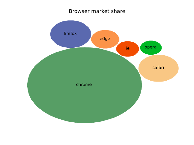
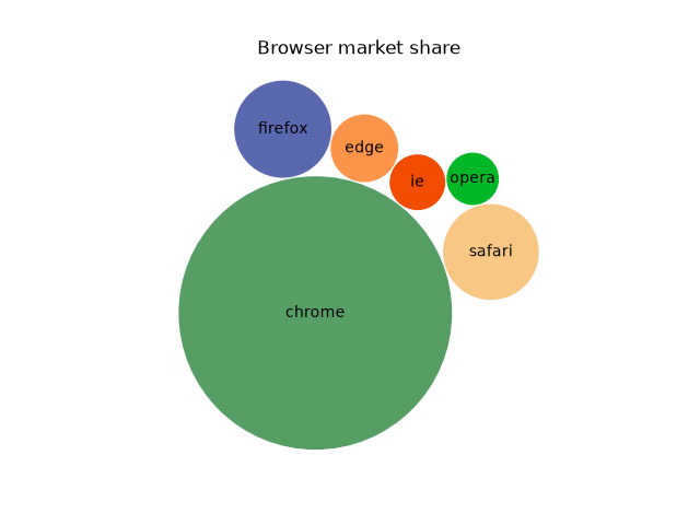
misc/patheffect_demo
===============
Source
"""
===============
Patheffect Demo
===============

"""
import matplotlib.pyplot as plt
import numpy as np

from matplotlib import patheffects

fig, (ax1, ax2, ax3) = plt.subplots(1, 3, figsize=(8, 3))
ax1.imshow([[1, 2], [2, 3]])
txt = ax1.annotate("test", (1., 1.), (0., 0),
                   arrowprops=dict(arrowstyle="->",
                                   connectionstyle="angle3", lw=2),
                   size=20, ha="center",
                   path_effects=[patheffects.withStroke(linewidth=3,
                                                        foreground="w")])
txt.arrow_patch.set_path_effects([
    patheffects.Stroke(linewidth=5, foreground="w"),
    patheffects.Normal()])

pe = [patheffects.withStroke(linewidth=3,
                             foreground="w")]
ax1.grid(True, linestyle="-", path_effects=pe)

arr = np.arange(25).reshape((5, 5))
ax2.imshow(arr)
cntr = ax2.contour(arr, colors="k")

cntr.set(path_effects=[patheffects.withStroke(linewidth=3, foreground="w")])

clbls = ax2.clabel(cntr, fmt="%2.0f", use_clabeltext=True)
plt.setp(clbls, path_effects=[
    patheffects.withStroke(linewidth=3, foreground="w")])

# shadow as a path effect
p1, = ax3.plot([0, 1], [0, 1])
leg = ax3.legend([p1], ["Line 1"], fancybox=True, loc='upper left')
leg.legendPatch.set_path_effects([patheffects.withSimplePatchShadow()])

plt.show()
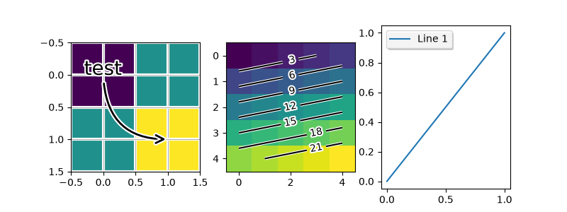
misc/print_stdout_sgskip
=====================
Source
"""
=====================
Print image to stdout
=====================

print png to standard out

usage: python print_stdout.py > somefile.png

"""

import sys

import matplotlib

matplotlib.use('Agg')
import matplotlib.pyplot as plt

plt.plot([1, 2, 3])
plt.savefig(sys.stdout.buffer)
misc/rasterization_demo
=================================
Source
"""
=================================
Rasterization for vector graphics
=================================

Rasterization converts vector graphics into a raster image (pixels). It can
speed up rendering and produce smaller files for large data sets, but comes
at the cost of a fixed resolution.

Whether rasterization should be used can be specified per artist.  This can be
useful to reduce the file size of large artists, while maintaining the
advantages of vector graphics for other artists such as the Axes
and text.  For instance a complicated `~.Axes.pcolormesh` or
`~.Axes.contourf` can be made significantly simpler by rasterizing.
Setting rasterization only affects vector backends such as PDF, SVG, or PS.

Rasterization is disabled by default. There are two ways to enable it, which
can also be combined:

- Set `~.Artist.set_rasterized` on individual artists, or use the keyword
  argument *rasterized* when creating the artist.
- Set `.Axes.set_rasterization_zorder` to rasterize all artists with a zorder
  less than the given value.

The storage size and the resolution of the rasterized artist is determined by
its physical size and the value of the ``dpi`` parameter passed to
`~.Figure.savefig`.

.. note::

    The image of this example shown in the HTML documentation is not a vector
    graphic. Therefore, it cannot illustrate the rasterization effect. Please
    run this example locally and check the generated graphics files.

"""

import matplotlib.pyplot as plt
import numpy as np

d = np.arange(100).reshape(10, 10)  # the values to be color-mapped
x, y = np.meshgrid(np.arange(11), np.arange(11))

theta = 0.25*np.pi
xx = x*np.cos(theta) - y*np.sin(theta)  # rotate x by -theta
yy = x*np.sin(theta) + y*np.cos(theta)  # rotate y by -theta

fig, ((ax1, ax2), (ax3, ax4)) = plt.subplots(2, 2, layout="constrained")

# pcolormesh without rasterization
ax1.set_aspect(1)
ax1.pcolormesh(xx, yy, d)
ax1.set_title("No Rasterization")

# pcolormesh with rasterization; enabled by keyword argument
ax2.set_aspect(1)
ax2.set_title("Rasterization")
ax2.pcolormesh(xx, yy, d, rasterized=True)

# pcolormesh with an overlaid text without rasterization
ax3.set_aspect(1)
ax3.pcolormesh(xx, yy, d)
ax3.text(0.5, 0.5, "Text", alpha=0.2,
         va="center", ha="center", size=50, transform=ax3.transAxes)
ax3.set_title("No Rasterization")

# pcolormesh with an overlaid text without rasterization; enabled by zorder.
# Setting the rasterization zorder threshold to 0 and a negative zorder on the
# pcolormesh rasterizes it. All artists have a non-negative zorder by default,
# so they (e.g. the text here) are not affected.
ax4.set_aspect(1)
m = ax4.pcolormesh(xx, yy, d, zorder=-10)
ax4.text(0.5, 0.5, "Text", alpha=0.2,
         va="center", ha="center", size=50, transform=ax4.transAxes)
ax4.set_rasterization_zorder(0)
ax4.set_title("Rasterization z$<-10$")

# Save files in pdf and eps format
plt.savefig("test_rasterization.pdf", dpi=150)
plt.savefig("test_rasterization.eps", dpi=150)

if not plt.rcParams["text.usetex"]:
    plt.savefig("test_rasterization.svg", dpi=150)
    # svg backend currently ignores the dpi

# %%
#
# .. admonition:: References
#
#    The use of the following functions, methods, classes and modules is shown
#    in this example:
#
#    - `matplotlib.artist.Artist.set_rasterized`
#    - `matplotlib.axes.Axes.set_rasterization_zorder`
#    - `matplotlib.axes.Axes.pcolormesh` / `matplotlib.pyplot.pcolormesh`
ValueError: unsupported format: 'eps' (use 'png', 'svg', 'pdf', or 'webp')
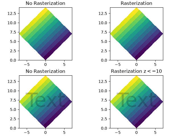
misc/set_and_get
======================
Source
"""
======================
Set and get properties
======================

The pyplot interface allows you to use ``setp`` and ``getp`` to
set and get object properties respectively, as well as to do
introspection on the object.

Setting with ``setp``
=====================

To set the linestyle of a line to be dashed, you use ``setp``::

  >>> line, = plt.plot([1, 2, 3])
  >>> plt.setp(line, linestyle='--')

If you want to know the valid types of arguments, you can provide the
name of the property you want to set without a value::

  >>> plt.setp(line, 'linestyle')
      linestyle: {'-', '--', '-.', ':', '', (offset, on-off-seq), ...}

If you want to see all the properties that can be set, and their
possible values, you can do::

    >>> plt.setp(line)

``setp`` operates on a single instance or a list of instances.  If you
are in query mode introspecting the possible values, only the first
instance in the sequence is used.  When actually setting values, all
the instances will be set.  For example, suppose you have a list of
two lines, the following will make both lines thicker and red::

    >>> x = np.arange(0, 1, 0.01)
    >>> y1 = np.sin(2*np.pi*x)
    >>> y2 = np.sin(4*np.pi*x)
    >>> lines = plt.plot(x, y1, x, y2)
    >>> plt.setp(lines, linewidth=2, color='r')


Getting with ``getp``
=====================

``getp`` returns the value of a given attribute.  You can use it to query
the value of a single attribute::

    >>> plt.getp(line, 'linewidth')
        0.5

or all the attribute/value pairs::

    >>> plt.getp(line)
        aa = True
        alpha = 1.0
        antialiased = True
        c = b
        clip_on = True
        color = b
        ... long listing skipped ...

Aliases
=======

To reduce keystrokes in interactive mode, a number of properties
have short aliases, e.g., 'lw' for 'linewidth' and 'mec' for
'markeredgecolor'.  When calling set or get in introspection mode,
these properties will be listed as 'fullname' or 'aliasname'.
"""


import matplotlib.pyplot as plt
import numpy as np

x = np.arange(0, 1.0, 0.01)
y1 = np.sin(2*np.pi*x)
y2 = np.sin(4*np.pi*x)
lines = plt.plot(x, y1, x, y2)
l1, l2 = lines
plt.setp(lines, linestyle='--')       # set both to dashed
plt.setp(l1, linewidth=2, color='r')  # line1 is thick and red
plt.setp(l2, linewidth=1, color='g')  # line2 is thinner and green


print('Line setters')
plt.setp(l1)
print('Line getters')
plt.getp(l1)

print('Rectangle setters')
plt.setp(plt.gca().patch)
print('Rectangle getters')
plt.getp(plt.gca().patch)

t = plt.title('Hi mom')
print('Text setters')
plt.setp(t)
print('Text getters')
plt.getp(t)

plt.show()
misc/svg_filter_line
==========================
Source
"""
==========================
Apply SVG filter to a line
==========================
Demonstrate SVG filtering effects which might be used with Matplotlib.
Note that the filtering effects are only effective if your SVG renderer
support it.
"""
import io
import xml.etree.ElementTree as ET
import matplotlib.pyplot as plt
import matplotlib.transforms as mtransforms
fig1 = plt.figure()
ax = fig1.add_axes((0.1, 0.1, 0.8, 0.8))
# draw lines
l1, = ax.plot([0.1, 0.5, 0.9], [0.1, 0.9, 0.5], "bo-",
mec="b", lw=5, ms=10, label="Line 1")
l2, = ax.plot([0.1, 0.5, 0.9], [0.5, 0.2, 0.7], "rs-",
mec="r", lw=5, ms=10, label="Line 2")
for l in [l1, l2]:
# draw shadows with same lines with slight offset and gray colors.
xx = l.get_xdata()
yy = l.get_ydata()
shadow, = ax.plot(xx, yy)
shadow.update_from(l)
# adjust color
shadow.set_color("0.2")
# adjust zorder of the shadow lines so that it is drawn below the
# original lines
shadow.set_zorder(l.get_zorder() - 0.5)
# offset transform
transform = mtransforms.offset_copy(l.get_transform(), fig1,
x=4.0, y=-6.0, units='points')
shadow.set_transform(transform)
# set the id for a later use
shadow.set_gid(l.get_label() + "_shadow")
ax.set_xlim(0., 1.)
ax.set_ylim(0., 1.)
# save the figure as a bytes string in the svg format.
f = io.BytesIO()
plt.savefig(f, format="svg")
# filter definition for a gaussian blur
filter_def = """
<defs xmlns='http://www.w3.org/2000/svg'
xmlns:xlink='http://www.w3.org/1999/xlink'>
<filter id='dropshadow' height='1.2' width='1.2'>
<feGaussianBlur result='blur' stdDeviation='3'/>
</filter>
</defs>
"""
# read in the saved svg
tree, xmlid = ET.XMLID(f.getvalue())
# insert the filter definition in the svg dom tree.
tree.insert(0, ET.XML(filter_def))
for l in [l1, l2]:
# pick up the svg element with given id
shadow = xmlid[l.get_label() + "_shadow"]
# apply shadow filter
shadow.set("filter", 'url(#dropshadow)')
fn = "svg_filter_line.svg"
print(f"Saving '{fn}'")
ET.ElementTree(tree).write(fn)
KeyError: 'Line 1_shadow'
misc/svg_filter_pie
==============
Source
"""
==============
SVG filter pie
==============
Demonstrate SVG filtering effects which might be used with Matplotlib.
The pie chart drawing code is borrowed from pie_demo.py
Note that the filtering effects are only effective if your SVG renderer
support it.
"""
import io
import xml.etree.ElementTree as ET
import matplotlib.pyplot as plt
from matplotlib.patches import Shadow
# make a square figure and Axes
fig = plt.figure(figsize=(6, 6))
ax = fig.add_axes((0.1, 0.1, 0.8, 0.8))
labels = 'Frogs', 'Hogs', 'Dogs', 'Logs'
fracs = [15, 30, 45, 10]
explode = (0, 0.05, 0, 0)
# We want to draw the shadow for each pie, but we will not use "shadow"
# option as it doesn't save the references to the shadow patches.
pie = ax.pie(fracs, explode=explode, labels=labels, autopct='%1.1f%%')
for w in pie.wedges:
# set the id with the label.
w.set_gid(w.get_label())
# we don't want to draw the edge of the pie
w.set_edgecolor("none")
for w in pie.wedges:
# create shadow patch
s = Shadow(w, -0.01, -0.01)
s.set_gid(w.get_gid() + "_shadow")
s.set_zorder(w.get_zorder() - 0.1)
ax.add_patch(s)
# save
f = io.BytesIO()
plt.savefig(f, format="svg")
# Filter definition for shadow using a gaussian blur and lighting effect.
# The lighting filter is copied from http://www.w3.org/TR/SVG/filters.html
# I tested it with Inkscape and Firefox3. "Gaussian blur" is supported
# in both, but the lighting effect only in Inkscape. Also note
# that, Inkscape's exporting also may not support it.
filter_def = """
<defs xmlns='http://www.w3.org/2000/svg'
xmlns:xlink='http://www.w3.org/1999/xlink'>
<filter id='dropshadow' height='1.2' width='1.2'>
<feGaussianBlur result='blur' stdDeviation='2'/>
</filter>
<filter id='MyFilter' filterUnits='objectBoundingBox'
x='0' y='0' width='1' height='1'>
<feGaussianBlur in='SourceAlpha' stdDeviation='4%' result='blur'/>
<feOffset in='blur' dx='4%' dy='4%' result='offsetBlur'/>
<feSpecularLighting in='blur' surfaceScale='5' specularConstant='.75'
specularExponent='20' lighting-color='#bbbbbb' result='specOut'>
<fePointLight x='-5000%' y='-10000%' z='20000%'/>
</feSpecularLighting>
<feComposite in='specOut' in2='SourceAlpha'
operator='in' result='specOut'/>
<feComposite in='SourceGraphic' in2='specOut' operator='arithmetic'
k1='0' k2='1' k3='1' k4='0'/>
</filter>
</defs>
"""
tree, xmlid = ET.XMLID(f.getvalue())
# insert the filter definition in the svg dom tree.
tree.insert(0, ET.XML(filter_def))
for i, pie_name in enumerate(labels):
pie = xmlid[pie_name]
pie.set("filter", 'url(#MyFilter)')
shadow = xmlid[pie_name + "_shadow"]
shadow.set("filter", 'url(#dropshadow)')
fn = "svg_filter_pie.svg"
print(f"Saving '{fn}'")
ET.ElementTree(tree).write(fn)
KeyError: 'Frogs'
misc/table_demo
==========
Source
"""
==========
Table Demo
==========
Demo of table function to display a table within a plot.
"""
import matplotlib.pyplot as plt
import numpy as np
data = [[ 66386, 174296, 75131, 577908, 32015],
[ 58230, 381139, 78045, 99308, 160454],
[ 89135, 80552, 152558, 497981, 603535],
[ 78415, 81858, 150656, 193263, 69638],
[139361, 331509, 343164, 781380, 52269]]
columns = ('Freeze', 'Wind', 'Flood', 'Quake', 'Hail')
rows = ['%d year' % x for x in (100, 50, 20, 10, 5)]
values = np.arange(0, 2500, 500)
value_increment = 1000
# Get some pastel shades for the colors
colors = plt.colormaps["BuPu"](np.linspace(0, 0.5, len(rows)))
n_rows = len(data)
index = np.arange(len(columns)) + 0.3
bar_width = 0.4
# Initialize the vertical-offset for the stacked bar chart.
y_offset = np.zeros(len(columns))
# Plot bars and create text labels for the table
cell_text = []
for row in range(n_rows):
plt.bar(index, data[row], bar_width, bottom=y_offset, color=colors[row])
y_offset = y_offset + data[row]
cell_text.append(['%1.1f' % (x / 1000.0) for x in y_offset])
# Reverse colors and text labels to display the last value at the top.
colors = colors[::-1]
cell_text.reverse()
# Add a table at the bottom of the Axes
the_table = plt.table(cellText=cell_text,
rowLabels=rows,
rowColours=colors,
colLabels=columns,
loc='bottom')
# Adjust layout to make room for the table:
plt.subplots_adjust(left=0.2, bottom=0.2)
plt.ylabel(f"Loss in ${value_increment}'s")
plt.yticks(values * value_increment, ['%d' % val for val in values])
plt.xticks([])
plt.title('Loss by Disaster')
plt.show()
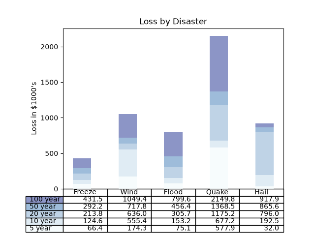
misc/tickedstroke_demo
=======================
Source
"""
=======================
TickedStroke patheffect
=======================
Matplotlib's :mod:`.patheffects` can be used to alter the way paths
are drawn at a low enough level that they can affect almost anything.
The :ref:`patheffects guide<patheffects_guide>`
details the use of patheffects.
The `~matplotlib.patheffects.TickedStroke` patheffect illustrated here
draws a path with a ticked style. The spacing, length, and angle of
ticks can be controlled.
See also the :doc:`/gallery/lines_bars_and_markers/lines_with_ticks_demo` example.
See also the :doc:`/gallery/images_contours_and_fields/contours_in_optimization_demo`
example.
"""
import matplotlib.pyplot as plt
import numpy as np
# %%
# Applying TickedStroke to paths
# ==============================
import matplotlib.patches as patches
from matplotlib.path import Path
import matplotlib.patheffects as patheffects
fig, ax = plt.subplots(figsize=(6, 6))
path = Path.unit_circle()
patch = patches.PathPatch(path, facecolor='none', lw=2, path_effects=[
patheffects.withTickedStroke(angle=-90, spacing=10, length=1)])
ax.add_patch(patch)
ax.axis('equal')
ax.set_xlim(-2, 2)
ax.set_ylim(-2, 2)
plt.show()
# %%
# Applying TickedStroke to lines
# ==============================
fig, ax = plt.subplots(figsize=(6, 6))
ax.plot([0, 1], [0, 1], label="Line",
path_effects=[patheffects.withTickedStroke(spacing=7, angle=135)])
nx = 101
x = np.linspace(0.0, 1.0, nx)
y = 0.3*np.sin(x*8) + 0.4
ax.plot(x, y, label="Curve", path_effects=[patheffects.withTickedStroke()])
ax.legend()
plt.show()
# %%
# Applying TickedStroke to contour plots
# ======================================
#
# Contour plot with objective and constraints.
# Curves generated by contour to represent a typical constraint in an
# optimization problem should be plotted with angles between zero and
# 180 degrees.
fig, ax = plt.subplots(figsize=(6, 6))
nx = 101
ny = 105
# Set up survey vectors
xvec = np.linspace(0.001, 4.0, nx)
yvec = np.linspace(0.001, 4.0, ny)
# Set up survey matrices. Design disk loading and gear ratio.
x1, x2 = np.meshgrid(xvec, yvec)
# Evaluate some stuff to plot
obj = x1**2 + x2**2 - 2*x1 - 2*x2 + 2
g1 = -(3*x1 + x2 - 5.5)
g2 = -(x1 + 2*x2 - 4.5)
g3 = 0.8 + x1**-3 - x2
cntr = ax.contour(x1, x2, obj, [0.01, 0.1, 0.5, 1, 2, 4, 8, 16],
colors='black')
ax.clabel(cntr, fmt="%2.1f", use_clabeltext=True)
cg1 = ax.contour(x1, x2, g1, [0], colors='sandybrown')
cg1.set(path_effects=[patheffects.withTickedStroke(angle=135)])
cg2 = ax.contour(x1, x2, g2, [0], colors='orangered')
cg2.set(path_effects=[patheffects.withTickedStroke(angle=60, length=2)])
cg3 = ax.contour(x1, x2, g3, [0], colors='mediumblue')
cg3.set(path_effects=[patheffects.withTickedStroke(spacing=7)])
ax.set_xlim(0, 4)
ax.set_ylim(0, 4)
plt.show()
# %%
# Direction/side of the ticks
# ===========================
#
# To change which side of the line the ticks are drawn, change the sign of the angle.
fig, ax = plt.subplots(figsize=(6, 6))
line_x = line_y = [0, 1]
ax.plot(line_x, line_y, label="Line",
path_effects=[patheffects.withTickedStroke(spacing=7, angle=135)])
ax.plot(line_x, line_y, label="Opposite side",
path_effects=[patheffects.withTickedStroke(spacing=7, angle=-135)])
ax.legend()
plt.show()
misc/transoffset
======================
Source
"""
======================
transforms.offset_copy
======================
This illustrates the use of `.transforms.offset_copy` to
make a transform that positions a drawing element such as
a text string at a specified offset in screen coordinates
(dots or inches) relative to a location given in any
coordinates.
Every Artist (Text, Line2D, etc.) has a transform that can be
set when the Artist is created, such as by the corresponding
pyplot function. By default, this is usually the Axes.transData
transform, going from data units to screen pixels. We can
use the `.offset_copy` function to make a modified copy of
this transform, where the modification consists of an
offset.
"""
import matplotlib.pyplot as plt
import numpy as np
import matplotlib.transforms as mtransforms
xs = np.arange(7)
ys = xs**2
fig = plt.figure(figsize=(5, 10))
ax = plt.subplot(2, 1, 1)
# If we want the same offset for each text instance,
# we only need to make one transform. To get the
# transform argument to offset_copy, we need to make the Axes
# first; the subplot function above is one way to do this.
trans_offset = mtransforms.offset_copy(ax.transData, fig=fig,
x=0.05, y=0.10, units='inches')
for x, y in zip(xs, ys):
plt.plot(x, y, 'ro')
plt.text(x, y, '%d, %d' % (int(x), int(y)), transform=trans_offset)
# offset_copy works for polar plots also.
ax = plt.subplot(2, 1, 2, projection='polar')
trans_offset = mtransforms.offset_copy(ax.transData, fig=fig,
y=6, units='dots')
for x, y in zip(xs, ys):
plt.polar(x, y, 'ro')
plt.text(x, y, '%d, %d' % (int(x), int(y)),
transform=trans_offset,
horizontalalignment='center',
verticalalignment='bottom')
plt.show()
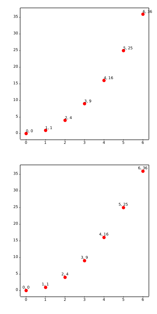
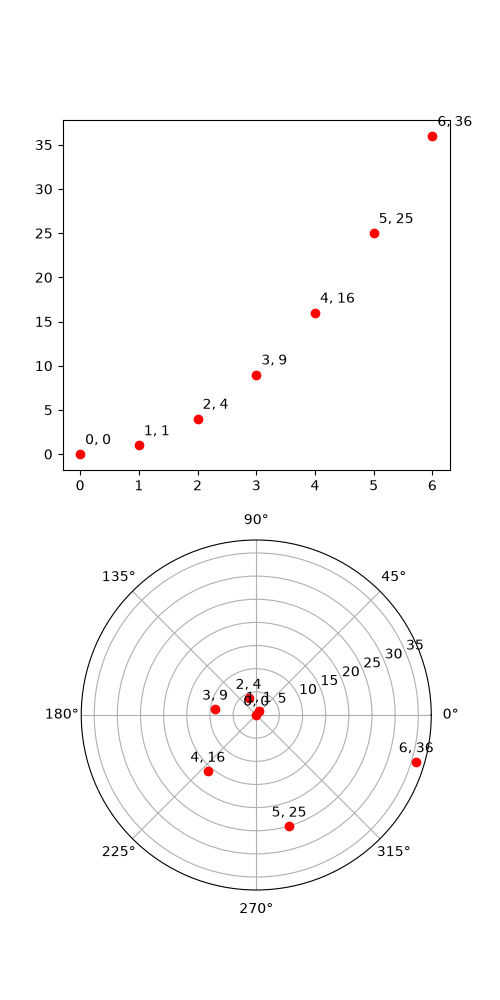
misc/zorder_demo
===========
Source
"""
===========
Zorder Demo
===========
The drawing order of artists is determined by their ``zorder`` attribute, which
is a floating point number. Artists with higher ``zorder`` are drawn on top.
You can change the order for individual artists by setting their ``zorder``.
The default value depends on the type of the Artist:
================================================================ =======
Artist Z-order
================================================================ =======
Images (`.AxesImage`, `.FigureImage`, `.BboxImage`) 0
`.Patch`, `.PatchCollection` 1
`.Line2D`, `.LineCollection` (including minor ticks, grid lines) 2
Major ticks 2.01
`.Text` (including Axes labels and titles) 3
`.Legend` 5
================================================================ =======
Any call to a plotting method can set a value for the zorder of that particular
item explicitly.
.. note::
`~.axes.Axes.set_axisbelow` and :rc:`axes.axisbelow` are convenient helpers
for setting the zorder of ticks and grid lines.
Drawing is done per `~.axes.Axes` at a time. If you have overlapping Axes, all
elements of the second Axes are drawn on top of the first Axes, irrespective of
their relative zorder.
"""
import matplotlib.pyplot as plt
import numpy as np
r = np.linspace(0.3, 1, 30)
theta = np.linspace(0, 4*np.pi, 30)
x = r * np.sin(theta)
y = r * np.cos(theta)
# %%
# The following example contains a `.Line2D` created by `~.axes.Axes.plot()`
# and the dots (a `.PatchCollection`) created by `~.axes.Axes.scatter()`.
# Hence, by default the dots are below the line (first subplot).
# In the second subplot, the ``zorder`` is set explicitly to move the dots
# on top of the line.
fig, (ax1, ax2) = plt.subplots(1, 2, figsize=(6, 3.2))
ax1.plot(x, y, 'C3', lw=3)
ax1.scatter(x, y, s=120)
ax1.set_title('Lines on top of dots')
ax2.plot(x, y, 'C3', lw=3)
ax2.scatter(x, y, s=120, zorder=2.5) # move dots on top of line
ax2.set_title('Dots on top of lines')
plt.tight_layout()
# %%
# Many functions that create a visible object accepts a ``zorder`` parameter.
# Alternatively, you can call ``set_zorder()`` on the created object later.
x = np.linspace(0, 7.5, 100)
plt.rcParams['lines.linewidth'] = 5
plt.figure()
plt.plot(x, np.sin(x), label='zorder=2', zorder=2) # bottom
plt.plot(x, np.sin(x+0.5), label='zorder=3', zorder=3)
plt.axhline(0, label='zorder=2.5', color='lightgrey', zorder=2.5)
plt.title('Custom order of elements')
l = plt.legend(loc='upper right')
l.set_zorder(2.5) # legend between blue and orange line
plt.show()
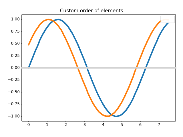
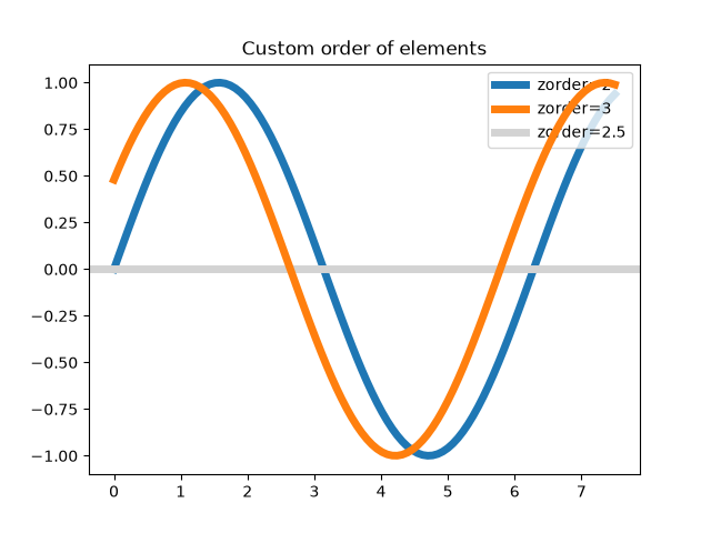
mplot3d/2dcollections3d
=======================
Source
"""
=======================
Plot 2D data on 3D plot
=======================
Demonstrates using ax.plot's *zdir* keyword to plot 2D data on
selective axes of a 3D plot.
"""
import matplotlib.pyplot as plt
import numpy as np
ax = plt.figure().add_subplot(projection='3d')
# Plot a sin curve using the x and y axes.
x = np.linspace(0, 1, 100)
y = np.sin(x * 2 * np.pi) / 2 + 0.5
ax.plot(x, y, zs=0, zdir='z', label='curve in (x, y)')
# Plot scatterplot data (20 2D points per colour) on the x and z axes.
colors = ('r', 'g', 'b', 'k')
# Fixing random state for reproducibility
np.random.seed(19680801)
x = np.random.sample(20 * len(colors))
y = np.random.sample(20 * len(colors))
c_list = []
for c in colors:
c_list.extend([c] * 20)
# By using zdir='y', the y value of these points is fixed to the zs value 0
# and the (x, y) points are plotted on the x and z axes.
ax.scatter(x, y, zs=0, zdir='y', c=c_list, label='points in (x, z)')
# Make legend, set axes limits and labels
ax.legend()
ax.set_xlim(0, 1)
ax.set_ylim(0, 1)
ax.set_zlim(0, 1)
ax.set_xlabel('X')
ax.set_ylabel('Y')
ax.set_zlabel('Z')
# Customize the view angle so it's easier to see that the scatter points lie
# on the plane y=0
ax.view_init(elev=20., azim=-35, roll=0)
plt.show()
# %%
# .. tags::
# plot-type: 3D, plot-type: scatter, plot-type: line,
# component: axes,
# level: intermediate
mplot3d is out of scope
mplot3d/3d_bars
=====================
Source
"""
=====================
Demo of 3D bar charts
=====================
A basic demo of how to plot 3D bars with and without shading.
"""
import matplotlib.pyplot as plt
import numpy as np
# set up the figure and Axes
fig = plt.figure(figsize=(8, 3))
ax1 = fig.add_subplot(121, projection='3d')
ax2 = fig.add_subplot(122, projection='3d')
# fake data
_x = np.arange(4)
_y = np.arange(5)
_xx, _yy = np.meshgrid(_x, _y)
x, y = _xx.ravel(), _yy.ravel()
top = x + y
bottom = np.zeros_like(top)
width = depth = 1
ax1.bar3d(x, y, bottom, width, depth, top, shade=True)
ax1.set_title('Shaded')
ax2.bar3d(x, y, bottom, width, depth, top, shade=False)
ax2.set_title('Not Shaded')
plt.show()
# %%
# .. tags::
# plot-type: 3D,
# styling: texture,
# plot-type: bar,
# level: beginner
mplot3d is out of scope
mplot3d/axlim_clip
=====================================
Source
"""
=====================================
Clip the data to the axes view limits
=====================================
Demonstrate clipping of line and marker data to the axes view limits. The
``axlim_clip`` keyword argument can be used in any of the 3D plotting
functions.
"""
import matplotlib.pyplot as plt
import numpy as np
fig, ax = plt.subplots(subplot_kw={"projection": "3d"})
# Make the data
x = np.arange(-5, 5, 0.5)
y = np.arange(-5, 5, 0.5)
X, Y = np.meshgrid(x, y)
R = np.sqrt(X**2 + Y**2)
Z = np.sin(R)
# Default behavior is axlim_clip=False
ax.plot_wireframe(X, Y, Z, color='C0')
# When axlim_clip=True, note that when a line segment has one vertex outside
# the view limits, the entire line is hidden. The same is true for 3D patches
# if one of their vertices is outside the limits (not shown).
ax.plot_wireframe(X, Y, Z, color='C1', axlim_clip=True)
# In this example, data where x < 0 or z > 0.5 is clipped
ax.set(xlim=(0, 10), ylim=(-5, 5), zlim=(-1, 0.5))
ax.legend(['axlim_clip=False (default)', 'axlim_clip=True'])
plt.show()
# %%
# .. tags::
# plot-type: 3D,
# level: beginner
mplot3d is out of scope
mplot3d/bars3d
========================================
Source
"""
========================================
Create 2D bar graphs in different planes
========================================
Demonstrates making a 3D plot which has 2D bar graphs projected onto
planes y=0, y=1, etc.
"""
import matplotlib.pyplot as plt
import numpy as np
# Fixing random state for reproducibility
np.random.seed(19680801)
fig = plt.figure()
ax = fig.add_subplot(projection='3d')
colors = ['r', 'g', 'b', 'y']
yticks = [3, 2, 1, 0]
for c, k in zip(colors, yticks):
# Generate the random data for the y=k 'layer'.
xs = np.arange(20)
ys = np.random.rand(20)
# You can provide either a single color or an array with the same length as
# xs and ys. To demonstrate this, we color the first bar of each set cyan.
cs = [c] * len(xs)
cs[0] = 'c'
# Plot the bar graph given by xs and ys on the plane y=k with 80% opacity.
ax.bar(xs, ys, zs=k, zdir='y', color=cs, alpha=0.8)
ax.set_xlabel('X')
ax.set_ylabel('Y')
ax.set_zlabel('Z')
# On the y-axis let's only label the discrete values that we have data for.
ax.set_yticks(yticks)
plt.show()
# %%
# .. tags::
# plot-type: 3D, plot-type: bar,
# styling: color,
# level: beginner
mplot3d is out of scope
mplot3d/box3d
===================
Source
"""
===================
3D box surface plot
===================
Given data on a gridded volume ``X``, ``Y``, ``Z``, this example plots the
data values on the volume surfaces.
The strategy is to select the data from each surface and plot
contours separately using `.axes3d.Axes3D.contourf` with appropriate
parameters *zdir* and *offset*.
"""
import matplotlib.pyplot as plt
import numpy as np
# Define dimensions
Nx, Ny, Nz = 100, 300, 500
X, Y, Z = np.meshgrid(np.arange(Nx), np.arange(Ny), -np.arange(Nz))
# Create fake data
data = (((X+100)**2 + (Y-20)**2 + 2*Z)/1000+1)
kw = {
'vmin': data.min(),
'vmax': data.max(),
'levels': np.linspace(data.min(), data.max(), 10),
}
# Create a figure with 3D ax
fig = plt.figure(figsize=(5, 4))
ax = fig.add_subplot(111, projection='3d')
# Plot contour surfaces
_ = ax.contourf(
X[:, :, 0], Y[:, :, 0], data[:, :, 0],
zdir='z', offset=0, **kw
)
_ = ax.contourf(
X[0, :, :], data[0, :, :], Z[0, :, :],
zdir='y', offset=0, **kw
)
C = ax.contourf(
data[:, -1, :], Y[:, -1, :], Z[:, -1, :],
zdir='x', offset=X.max(), **kw
)
# --
# Set limits of the plot from coord limits
xmin, xmax = X.min(), X.max()
ymin, ymax = Y.min(), Y.max()
zmin, zmax = Z.min(), Z.max()
ax.set(xlim=(xmin, xmax), ylim=(ymin, ymax), zlim=(zmin, zmax))
# Plot edges
edges_kw = dict(color='0.4', linewidth=1, zorder=1e3)
ax.plot([xmax, xmax], [ymin, ymax], 0, **edges_kw)
ax.plot([xmin, xmax], [ymin, ymin], 0, **edges_kw)
ax.plot([xmax, xmax], [ymin, ymin], [zmin, zmax], **edges_kw)
# Set labels and zticks
ax.set(
xlabel='X [km]',
ylabel='Y [km]',
zlabel='Z [m]',
zticks=[0, -150, -300, -450],
)
# Set zoom and angle view
ax.view_init(40, -30, 0)
ax.set_box_aspect(None, zoom=0.9)
# Colorbar
fig.colorbar(C, ax=ax, fraction=0.02, pad=0.1, label='Name [units]')
# Show Figure
plt.show()
# %%
# .. tags::
# plot-type: 3D,
# level: intermediate
mplot3d is out of scope
mplot3d/contour3d
=================================
Source
""" ================================= Plot contour (level) curves in 3D ================================= This is like a contour plot in 2D except that the ``f(x, y)=c`` curve is plotted on the plane ``z=c``. """ import matplotlib.pyplot as plt from mpl_toolkits.mplot3d import axes3d ax = plt.figure().add_subplot(projection='3d') X, Y, Z = axes3d.get_test_data(0.05) ax.contour(X, Y, Z, cmap="coolwarm") # Plot contour curves plt.show() # %% # .. tags:: # plot-type: 3D, # level: beginner
mplot3d is out of scope
mplot3d/contour3d_2
===========================================================
Source
""" =========================================================== Plot contour (level) curves in 3D using the extend3d option =========================================================== This modification of the :doc:`contour3d` example uses ``extend3d=True`` to extend the curves vertically into 'ribbons'. """ import matplotlib.pyplot as plt from mpl_toolkits.mplot3d import axes3d ax = plt.figure().add_subplot(projection='3d') X, Y, Z = axes3d.get_test_data(0.05) ax.contour(X, Y, Z, extend3d=True, cmap="coolwarm") plt.show() # %% # .. tags:: # plot-type: 3D, # level: beginner
mplot3d is out of scope
mplot3d/contour3d_3
=====================================
Source
"""
=====================================
Project contour profiles onto a graph
=====================================
Demonstrates displaying a 3D surface while also projecting contour 'profiles'
onto the 'walls' of the graph.
See :doc:`contourf3d_2` for the filled version.
"""
import matplotlib.pyplot as plt
from mpl_toolkits.mplot3d import axes3d
ax = plt.figure().add_subplot(projection='3d')
X, Y, Z = axes3d.get_test_data(0.05)
# Plot the 3D surface
ax.plot_surface(X, Y, Z, edgecolor='royalblue', lw=0.5, rstride=8, cstride=8,
alpha=0.3)
# Plot projections of the contours for each dimension. By choosing offsets
# that match the appropriate axes limits, the projected contours will sit on
# the 'walls' of the graph.
ax.contour(X, Y, Z, zdir='z', offset=-100, cmap='coolwarm')
ax.contour(X, Y, Z, zdir='x', offset=-40, cmap='coolwarm')
ax.contour(X, Y, Z, zdir='y', offset=40, cmap='coolwarm')
ax.set(xlim=(-40, 40), ylim=(-40, 40), zlim=(-100, 100),
xlabel='X', ylabel='Y', zlabel='Z')
plt.show()
# %%
# .. tags::
# plot-type: 3D,
# component: axes,
# level: intermediate
mplot3d is out of scope
mplot3d/contourf3d
===============
Source
""" =============== Filled contours =============== `.Axes3D.contourf` differs from `.Axes3D.contour` in that it creates filled contours, i.e. a discrete number of colours are used to shade the domain. This is like a `.Axes.contourf` plot in 2D except that the shaded region corresponding to the level c is graphed on the plane ``z=c``. """ import matplotlib.pyplot as plt from mpl_toolkits.mplot3d import axes3d ax = plt.figure().add_subplot(projection='3d') X, Y, Z = axes3d.get_test_data(0.05) ax.contourf(X, Y, Z, cmap="coolwarm") plt.show() # %% # .. tags:: # plot-type: 3D, # level: beginner
mplot3d is out of scope
mplot3d/contourf3d_2
===================================
Source
"""
===================================
Project filled contour onto a graph
===================================
Demonstrates displaying a 3D surface while also projecting filled contour
'profiles' onto the 'walls' of the graph.
See :doc:`contour3d_3` for the unfilled version.
"""
import matplotlib.pyplot as plt
from mpl_toolkits.mplot3d import axes3d
ax = plt.figure().add_subplot(projection='3d')
X, Y, Z = axes3d.get_test_data(0.05)
# Plot the 3D surface
ax.plot_surface(X, Y, Z, edgecolor='royalblue', lw=0.5, rstride=8, cstride=8,
alpha=0.3)
# Plot projections of the contours for each dimension. By choosing offsets
# that match the appropriate axes limits, the projected contours will sit on
# the 'walls' of the graph
ax.contourf(X, Y, Z, zdir='z', offset=-100, cmap='coolwarm')
ax.contourf(X, Y, Z, zdir='x', offset=-40, cmap='coolwarm')
ax.contourf(X, Y, Z, zdir='y', offset=40, cmap='coolwarm')
ax.set(xlim=(-40, 40), ylim=(-40, 40), zlim=(-100, 100),
xlabel='X', ylabel='Y', zlabel='Z')
plt.show()
# %%
# .. tags::
# plot-type: 3D,
# component: axes,
# level: intermediate
mplot3d is out of scope
mplot3d/custom_shaded_3d_surface
=======================================
Source
"""
=======================================
Custom hillshading in a 3D surface plot
=======================================
Demonstrates using custom hillshading in a 3D surface plot.
"""
import matplotlib.pyplot as plt
import numpy as np
from matplotlib import cbook
from matplotlib.colors import LightSource
# Load and format data
dem = cbook.get_sample_data('jacksboro_fault_dem.npz')
z = dem['elevation']
nrows, ncols = z.shape
x = np.linspace(dem['xmin'], dem['xmax'], ncols)
y = np.linspace(dem['ymin'], dem['ymax'], nrows)
x, y = np.meshgrid(x, y)
region = np.s_[5:50, 5:50]
x, y, z = x[region], y[region], z[region]
# Set up plot
fig, ax = plt.subplots(subplot_kw=dict(projection='3d'))
ls = LightSource(270, 45)
# To use a custom hillshading mode, override the built-in shading and pass
# in the rgb colors of the shaded surface calculated from "shade".
rgb = ls.shade(z, cmap=plt.colormaps["gist_earth"], vert_exag=0.1, blend_mode='soft')
surf = ax.plot_surface(x, y, z, rstride=1, cstride=1, facecolors=rgb,
linewidth=0, antialiased=False, shade=False)
plt.show()
# %%
# .. tags::
# plot-type: 3D,
# level: intermediate,
# domain: cartography
mplot3d is out of scope
mplot3d/errorbar3d
============
Source
"""
============
3D errorbars
============
An example of using errorbars with upper and lower limits in mplot3d.
"""
import matplotlib.pyplot as plt
import numpy as np
ax = plt.figure().add_subplot(projection='3d')
# setting up a parametric curve
t = np.arange(0, 2*np.pi+.1, 0.01)
x, y, z = np.sin(t), np.cos(3*t), np.sin(5*t)
estep = 15
i = np.arange(t.size)
zuplims = (i % estep == 0) & (i // estep % 3 == 0)
zlolims = (i % estep == 0) & (i // estep % 3 == 2)
ax.errorbar(x, y, z, 0.2, zuplims=zuplims, zlolims=zlolims, errorevery=estep)
ax.set_xlabel("X label")
ax.set_ylabel("Y label")
ax.set_zlabel("Z label")
plt.show()
# %%
# .. tags::
# plot-type: 3D,
# component: error,
# level: beginner
mplot3d is out of scope
mplot3d/fillbetween3d
=====================
Source
""" ===================== Fill between 3D lines ===================== Demonstrate how to fill the space between 3D lines with surfaces. Here we create a sort of "lampshade" shape. """ import matplotlib.pyplot as plt import numpy as np N = 50 theta = np.linspace(0, 2*np.pi, N) x1 = np.cos(theta) y1 = np.sin(theta) z1 = 0.1 * np.sin(6 * theta) x2 = 0.6 * np.cos(theta) y2 = 0.6 * np.sin(theta) z2 = 2 # Note that scalar values work in addition to length N arrays fig = plt.figure() ax = fig.add_subplot(projection='3d') ax.fill_between(x1, y1, z1, x2, y2, z2, alpha=0.5, edgecolor='k') plt.show() # %% # .. tags:: # plot-type: 3D, # plot-type: fill_between, # level: beginner
mplot3d is out of scope
mplot3d/fillunder3d
=========================
Source
"""
=========================
Fill under 3D line graphs
=========================
Demonstrate how to create polygons which fill the space under a line
graph. In this example polygons are semi-transparent, creating a sort
of 'jagged stained glass' effect.
"""
import math
import matplotlib.pyplot as plt
import numpy as np
gamma = np.vectorize(math.gamma)
N = 31
x = np.linspace(0., 10., N)
lambdas = range(1, 9)
ax = plt.figure().add_subplot(projection='3d')
facecolors = plt.colormaps['viridis_r'](np.linspace(0, 1, len(lambdas)))
for i, l in enumerate(lambdas):
# Note fill_between can take coordinates as length N vectors, or scalars
ax.fill_between(x, l, l**x * np.exp(-l) / gamma(x + 1),
x, l, 0,
facecolors=facecolors[i], alpha=.7)
ax.set(xlim=(0, 10), ylim=(1, 9), zlim=(0, 0.35),
xlabel='x', ylabel=r'$\lambda$', zlabel='probability')
plt.show()
# %%
# .. tags::
# plot-type: 3D,
# plot-type: fill_between,
# level: beginner
mplot3d is out of scope
mplot3d/hist3d
==============================
Source
""" ============================== Create 3D histogram of 2D data ============================== Demo of a histogram for 2D data as a bar graph in 3D. """ import matplotlib.pyplot as plt import numpy as np # Fixing random state for reproducibility np.random.seed(19680801) fig = plt.figure() ax = fig.add_subplot(projection='3d') x, y = np.random.rand(2, 100) * 4 hist, xedges, yedges = np.histogram2d(x, y, bins=4, range=[[0, 4], [0, 4]]) # Construct arrays for the anchor positions of the 16 bars. xpos, ypos = np.meshgrid(xedges[:-1] + 0.25, yedges[:-1] + 0.25, indexing="ij") xpos = xpos.ravel() ypos = ypos.ravel() zpos = 0 # Construct arrays with the dimensions for the 16 bars. dx = dy = 0.5 * np.ones_like(zpos) dz = hist.ravel() ax.bar3d(xpos, ypos, zpos, dx, dy, dz, zsort='average') plt.show() # %% # .. tags:: # plot-type: 3D, plot-type: histogram, # level: beginner
mplot3d is out of scope
mplot3d/imshow3d
===============
Source
"""
===============
2D images in 3D
===============
This example demonstrates how to plot 2D color coded images (similar to
`.Axes.imshow`) as a plane in 3D.
Matplotlib does not have a native function for this. Below we build one by relying
on `.Axes3D.plot_surface`. For simplicity, there are some differences to
`.Axes.imshow`: This function does not set the aspect of the Axes, hence pixels are
not necessarily square. Also, pixel edges are on integer values rather than pixel
centers. Furthermore, many optional parameters of `.Axes.imshow` are not implemented.
Multiple calls of ``imshow3d`` use independent norms and thus different color scales
by default. If you want to have a single common color scale, you need to construct
a suitable norm beforehand and pass it to all ``imshow3d`` calls.
A fundamental limitation of the 3D plotting engine is that intersecting objects cannot
be drawn correctly. One object will always be drawn after the other. Therefore,
multiple image planes can well be used in the background as shown in this example.
But this approach is not suitable if the planes intersect.
"""
import matplotlib.pyplot as plt
import numpy as np
from matplotlib.colors import Normalize
def imshow3d(ax, array, value_direction='z', pos=0, norm=None, cmap=None):
"""
Display a 2D array as a color-coded 2D image embedded in 3d.
The image will be in a plane perpendicular to the coordinate axis *value_direction*.
Parameters
----------
ax : Axes3D
The 3D Axes to plot into.
array : 2D numpy array
The image values.
value_direction : {'x', 'y', 'z'}
The axis normal to the image plane.
pos : float
The numeric value on the *value_direction* axis at which the image plane is
located.
norm : `~matplotlib.colors.Normalize`, default: Normalize
The normalization method used to scale scalar data. See `imshow()`.
cmap : str or `~matplotlib.colors.Colormap`, default: :rc:`image.cmap`
The Colormap instance or registered colormap name used to map scalar data
to colors.
"""
if norm is None:
norm = Normalize()
colors = plt.get_cmap(cmap)(norm(array))
if value_direction == 'x':
nz, ny = array.shape
zi, yi = np.mgrid[0:nz + 1, 0:ny + 1]
xi = np.full_like(yi, pos)
elif value_direction == 'y':
nx, nz = array.shape
xi, zi = np.mgrid[0:nx + 1, 0:nz + 1]
yi = np.full_like(zi, pos)
elif value_direction == 'z':
ny, nx = array.shape
yi, xi = np.mgrid[0:ny + 1, 0:nx + 1]
zi = np.full_like(xi, pos)
else:
raise ValueError(f"Invalid value_direction: {value_direction!r}")
ax.plot_surface(xi, yi, zi, rstride=1, cstride=1, facecolors=colors, shade=False)
fig = plt.figure()
ax = fig.add_subplot(projection='3d')
ax.set(xlabel="x", ylabel="y", zlabel="z")
nx, ny, nz = 8, 10, 5
data_xy = np.arange(ny * nx).reshape(ny, nx) + 15 * np.random.random((ny, nx))
data_yz = np.arange(nz * ny).reshape(nz, ny) + 10 * np.random.random((nz, ny))
data_zx = np.arange(nx * nz).reshape(nx, nz) + 8 * np.random.random((nx, nz))
imshow3d(ax, data_xy)
imshow3d(ax, data_yz, value_direction='x', cmap='magma')
imshow3d(ax, data_zx, value_direction='y', pos=ny, cmap='plasma')
plt.show()
# %%
# .. tags::
# plot-type: 3D,
# styling: colormap,
# level: advanced
mplot3d is out of scope
mplot3d/intersecting_planes
===================
Source
"""
===================
Intersecting planes
===================
This examples demonstrates drawing intersecting planes in 3D. It is a generalization
of :doc:`/gallery/mplot3d/imshow3d`.
Drawing intersecting planes in `.mplot3d` is complicated, because `.mplot3d` is not a
real 3D renderer, but only projects the Artists into 3D and draws them in the right
order. This does not work correctly if Artists overlap each other mutually. In this
example, we lift the problem of mutual overlap by segmenting the planes at their
intersections, making four parts out of each plane.
This examples only works correctly for planes that cut each other in halves. This
limitation is intentional to keep the code more readable. Cutting at arbitrary
positions would of course be possible but makes the code even more complex.
Thus, this example is more a demonstration of the concept how to work around
limitations of the 3D visualization, it's not a refined solution for drawing
arbitrary intersecting planes, which you can copy-and-paste as is.
"""
import matplotlib.pyplot as plt
import numpy as np
def plot_quadrants(ax, array, fixed_coord, cmap):
"""For a given 3d *array* plot a plane with *fixed_coord*, using four quadrants."""
nx, ny, nz = array.shape
index = {
'x': (nx // 2, slice(None), slice(None)),
'y': (slice(None), ny // 2, slice(None)),
'z': (slice(None), slice(None), nz // 2),
}[fixed_coord]
plane_data = array[index]
n0, n1 = plane_data.shape
quadrants = [
plane_data[:n0 // 2, :n1 // 2],
plane_data[:n0 // 2, n1 // 2:],
plane_data[n0 // 2:, :n1 // 2],
plane_data[n0 // 2:, n1 // 2:]
]
min_val = array.min()
max_val = array.max()
cmap = plt.get_cmap(cmap)
for i, quadrant in enumerate(quadrants):
facecolors = cmap((quadrant - min_val) / (max_val - min_val))
if fixed_coord == 'x':
Y, Z = np.mgrid[0:ny // 2, 0:nz // 2]
X = nx // 2 * np.ones_like(Y)
Y_offset = (i // 2) * ny // 2
Z_offset = (i % 2) * nz // 2
ax.plot_surface(X, Y + Y_offset, Z + Z_offset, rstride=1, cstride=1,
facecolors=facecolors, shade=False)
elif fixed_coord == 'y':
X, Z = np.mgrid[0:nx // 2, 0:nz // 2]
Y = ny // 2 * np.ones_like(X)
X_offset = (i // 2) * nx // 2
Z_offset = (i % 2) * nz // 2
ax.plot_surface(X + X_offset, Y, Z + Z_offset, rstride=1, cstride=1,
facecolors=facecolors, shade=False)
elif fixed_coord == 'z':
X, Y = np.mgrid[0:nx // 2, 0:ny // 2]
Z = nz // 2 * np.ones_like(X)
X_offset = (i // 2) * nx // 2
Y_offset = (i % 2) * ny // 2
ax.plot_surface(X + X_offset, Y + Y_offset, Z, rstride=1, cstride=1,
facecolors=facecolors, shade=False)
def figure_3D_array_slices(array, cmap=None):
"""Plot a 3d array using three intersecting centered planes."""
fig = plt.figure()
ax = fig.add_subplot(projection='3d')
ax.set_box_aspect(array.shape)
plot_quadrants(ax, array, 'x', cmap=cmap)
plot_quadrants(ax, array, 'y', cmap=cmap)
plot_quadrants(ax, array, 'z', cmap=cmap)
return fig, ax
nx, ny, nz = 70, 100, 50
r_square = (np.mgrid[-1:1:1j * nx, -1:1:1j * ny, -1:1:1j * nz] ** 2).sum(0)
figure_3D_array_slices(r_square, cmap='viridis_r')
plt.show()
# %%
# .. tags::
# plot-type: 3D,
# level: advanced
mplot3d is out of scope
mplot3d/lines3d
================
Source
""" ================ Parametric curve ================ This example demonstrates plotting a parametric curve in 3D. """ import matplotlib.pyplot as plt import numpy as np ax = plt.figure().add_subplot(projection='3d') # Prepare arrays x, y, z theta = np.linspace(-4 * np.pi, 4 * np.pi, 100) z = np.linspace(-2, 2, 100) r = z**2 + 1 x = r * np.sin(theta) y = r * np.cos(theta) ax.plot(x, y, z, label='parametric curve') ax.legend() plt.show() # %% # .. tags:: # plot-type: 3D, # level: beginner
mplot3d is out of scope
mplot3d/lorenz_attractor
================
Source
"""
================
Lorenz attractor
================
This is an example of plotting Edward Lorenz's 1963 `"Deterministic Nonperiodic
Flow"`_ in a 3-dimensional space using mplot3d.
.. _"Deterministic Nonperiodic Flow":
https://journals.ametsoc.org/view/journals/atsc/20/2/1520-0469_1963_020_0130_dnf_2_0_co_2.xml
.. note::
Because this is a simple non-linear ODE, it would be more easily done using
SciPy's ODE solver, but this approach depends only upon NumPy.
"""
import matplotlib.pyplot as plt
import numpy as np
def lorenz(xyz, *, s=10, r=28, b=2.667):
"""
Parameters
----------
xyz : array-like, shape (3,)
Point of interest in three-dimensional space.
s, r, b : float
Parameters defining the Lorenz attractor.
Returns
-------
xyz_dot : array, shape (3,)
Values of the Lorenz attractor's partial derivatives at *xyz*.
"""
x, y, z = xyz
x_dot = s*(y - x)
y_dot = r*x - y - x*z
z_dot = x*y - b*z
return np.array([x_dot, y_dot, z_dot])
dt = 0.01
num_steps = 10000
xyzs = np.empty((num_steps + 1, 3)) # Need one more for the initial values
xyzs[0] = (0., 1., 1.05) # Set initial values
# Step through "time", calculating the partial derivatives at the current point
# and using them to estimate the next point
for i in range(num_steps):
xyzs[i + 1] = xyzs[i] + lorenz(xyzs[i]) * dt
# Plot
ax = plt.figure().add_subplot(projection='3d')
ax.plot(*xyzs.T, lw=0.5)
ax.set_xlabel("X Axis")
ax.set_ylabel("Y Axis")
ax.set_zlabel("Z Axis")
ax.set_title("Lorenz Attractor")
plt.show()
# %%
# .. tags::
# plot-type: 3D,
# level: intermediate
mplot3d is out of scope
mplot3d/mixed_subplots
=============================
Source
"""
=============================
2D and 3D Axes in same figure
=============================
This example shows a how to plot a 2D and a 3D plot on the same figure.
"""
import matplotlib.pyplot as plt
import numpy as np
def f(t):
return np.cos(2*np.pi*t) * np.exp(-t)
# Set up a figure twice as tall as it is wide
fig = plt.figure(figsize=plt.figaspect(2.))
fig.suptitle('A tale of 2 subplots')
# First subplot
ax = fig.add_subplot(2, 1, 1)
t1 = np.arange(0.0, 5.0, 0.1)
t2 = np.arange(0.0, 5.0, 0.02)
t3 = np.arange(0.0, 2.0, 0.01)
ax.plot(t1, f(t1), 'bo',
t2, f(t2), 'k--', markerfacecolor='green')
ax.grid(True)
ax.set_ylabel('Damped oscillation')
# Second subplot
ax = fig.add_subplot(2, 1, 2, projection='3d')
X = np.arange(-5, 5, 0.25)
Y = np.arange(-5, 5, 0.25)
X, Y = np.meshgrid(X, Y)
R = np.sqrt(X**2 + Y**2)
Z = np.sin(R)
surf = ax.plot_surface(X, Y, Z, rstride=1, cstride=1,
linewidth=0, antialiased=False)
ax.set_zlim(-1, 1)
plt.show()
# %%
# .. tags::
# plot-type: 3D,
# component: subplot,
# level: beginner
mplot3d is out of scope
mplot3d/offset
=========================
Source
"""
=========================
Automatic text offsetting
=========================
This example demonstrates mplot3d's offset text display.
As one rotates the 3D figure, the offsets should remain oriented the
same way as the axis label, and should also be located "away"
from the center of the plot.
This demo triggers the display of the offset text for the x- and
y-axis by adding 1e5 to X and Y. Anything less would not
automatically trigger it.
"""
import matplotlib.pyplot as plt
import numpy as np
ax = plt.figure().add_subplot(projection='3d')
X, Y = np.mgrid[0:6*np.pi:0.25, 0:4*np.pi:0.25]
Z = np.sqrt(np.abs(np.cos(X) + np.cos(Y)))
ax.plot_surface(X + 1e5, Y + 1e5, Z, cmap='autumn', cstride=2, rstride=2)
ax.set_xlabel("X label")
ax.set_ylabel("Y label")
ax.set_zlabel("Z label")
ax.set_zlim(0, 2)
plt.show()
# %%
# .. tags::
# plot-type: 3D,
# component: label,
# interactivity: pan,
# level: beginner
mplot3d is out of scope
mplot3d/pathpatch3d
============================
Source
"""
============================
Draw flat objects in 3D plot
============================
Demonstrate using `.pathpatch_2d_to_3d` to 'draw' shapes and text on a 3D plot.
"""
import matplotlib.pyplot as plt
import numpy as np
from matplotlib.patches import Circle, PathPatch
from matplotlib.text import TextPath
from matplotlib.transforms import Affine2D
import mpl_toolkits.mplot3d.art3d as art3d
def text3d(ax, xyz, s, zdir="z", size=None, angle=0, usetex=False, **kwargs):
"""
Plots the string *s* on the Axes *ax*, with position *xyz*, size *size*,
and rotation angle *angle*. *zdir* gives the axis which is to be treated as
the third dimension. *usetex* is a boolean indicating whether the string
should be run through a LaTeX subprocess or not. Any additional keyword
arguments are forwarded to `.transform_path`.
Note: zdir affects the interpretation of xyz.
"""
x, y, z = xyz
if zdir == "y":
xy1, z1 = (x, z), y
elif zdir == "x":
xy1, z1 = (y, z), x
else:
xy1, z1 = (x, y), z
text_path = TextPath((0, 0), s, size=size, usetex=usetex)
trans = Affine2D().rotate(angle).translate(xy1[0], xy1[1])
p1 = PathPatch(trans.transform_path(text_path), **kwargs)
ax.add_patch(p1)
art3d.pathpatch_2d_to_3d(p1, z=z1, zdir=zdir)
fig = plt.figure()
ax = fig.add_subplot(projection='3d')
# Draw a circle on the x=0 'wall'
p = Circle((5, 5), 3)
ax.add_patch(p)
art3d.pathpatch_2d_to_3d(p, z=0, zdir="x")
# Manually label the axes
text3d(ax, (4, -2, 0), "X-axis", zdir="z", size=.5, usetex=False,
ec="none", fc="k")
text3d(ax, (12, 4, 0), "Y-axis", zdir="z", size=.5, usetex=False,
angle=np.pi / 2, ec="none", fc="k")
text3d(ax, (12, 10, 4), "Z-axis", zdir="y", size=.5, usetex=False,
angle=np.pi / 2, ec="none", fc="k")
# Write a Latex formula on the z=0 'floor'
text3d(ax, (1, 5, 0),
r"$\displaystyle G_{\mu\nu} + \Lambda g_{\mu\nu} = "
r"\frac{8\pi G}{c^4} T_{\mu\nu} $",
zdir="z", size=1, usetex=True,
ec="none", fc="k")
ax.set_xlim(0, 10)
ax.set_ylim(0, 10)
ax.set_zlim(0, 10)
plt.show()
# %%
# .. tags::
# plot-type: 3D,
# component: label,
# level: advanced
mplot3d is out of scope
mplot3d/polys3d
====================
Source
"""
====================
Generate 3D polygons
====================
Demonstrate how to create polygons in 3D. Here we stack 3 hexagons.
"""
import matplotlib.pyplot as plt
import numpy as np
from mpl_toolkits.mplot3d.art3d import Poly3DCollection
# Coordinates of a hexagon
angles = np.linspace(0, 2 * np.pi, 6, endpoint=False)
x = np.cos(angles)
y = np.sin(angles)
zs = [-3, -2, -1]
# Close the hexagon by repeating the first vertex
x = np.append(x, x[0])
y = np.append(y, y[0])
verts = []
for z in zs:
verts.append(list(zip(x*z, y*z, np.full_like(x, z))))
verts = np.array(verts)
ax = plt.figure().add_subplot(projection='3d')
poly = Poly3DCollection(verts, alpha=.7)
ax.add_collection3d(poly)
ax.set_aspect('equalxy')
plt.show()
# %%
# .. tags::
# plot-type: 3D,
# styling: colormap,
# level: intermediate
mplot3d is out of scope
mplot3d/projections
========================
Source
"""
========================
3D plot projection types
========================
Demonstrates the different camera projections for 3D plots, and the effects of
changing the focal length for a perspective projection. Note that Matplotlib
corrects for the 'zoom' effect of changing the focal length.
The default focal length of 1 corresponds to a Field of View (FOV) of 90 deg.
An increased focal length between 1 and infinity "flattens" the image, while a
decreased focal length between 1 and 0 exaggerates the perspective and gives
the image more apparent depth. In the limiting case, a focal length of
infinity corresponds to an orthographic projection after correction of the
zoom effect.
You can calculate focal length from a FOV via the equation:
.. math::
1 / \\tan (\\mathrm{FOV} / 2)
Or vice versa:
.. math::
\\mathrm{FOV} = 2 \\arctan (1 / \\mathrm{focal length})
"""
import matplotlib.pyplot as plt
from mpl_toolkits.mplot3d import axes3d
fig, axs = plt.subplots(1, 3, subplot_kw={'projection': '3d'})
# Get the test data
X, Y, Z = axes3d.get_test_data(0.05)
# Plot the data
for ax in axs:
ax.plot_wireframe(X, Y, Z, rstride=10, cstride=10)
# Set the orthographic projection.
axs[0].set_proj_type('ortho') # FOV = 0 deg
axs[0].set_title("'ortho'\nfocal_length = ∞", fontsize=10)
# Set the perspective projections
axs[1].set_proj_type('persp') # FOV = 90 deg
axs[1].set_title("'persp'\nfocal_length = 1 (default)", fontsize=10)
axs[2].set_proj_type('persp', focal_length=0.2) # FOV = 157.4 deg
axs[2].set_title("'persp'\nfocal_length = 0.2", fontsize=10)
plt.show()
# %%
# .. tags::
# plot-type: 3D,
# styling: small-multiples,
# component: subplot,
# level: intermediate
mplot3d is out of scope
mplot3d/quiver3d
==============
Source
"""
==============
3D quiver plot
==============
Demonstrates plotting directional arrows at points on a 3D meshgrid.
"""
import matplotlib.pyplot as plt
import numpy as np
ax = plt.figure().add_subplot(projection='3d')
# Make the grid
x, y, z = np.meshgrid(np.arange(-0.8, 1, 0.2),
np.arange(-0.8, 1, 0.2),
np.arange(-0.8, 1, 0.8))
# Make the direction data for the arrows
u = np.sin(np.pi * x) * np.cos(np.pi * y) * np.cos(np.pi * z)
v = -np.cos(np.pi * x) * np.sin(np.pi * y) * np.cos(np.pi * z)
w = (np.sqrt(2.0 / 3.0) * np.cos(np.pi * x) * np.cos(np.pi * y) *
np.sin(np.pi * z))
ax.quiver(x, y, z, u, v, w, length=0.1, normalize=True)
plt.show()
# %%
# .. tags::
# plot-type: 3D,
# level: beginner
mplot3d is out of scope
mplot3d/rotate_axes3d_sgskip
==================
Source
"""
==================
Rotating a 3D plot
==================
A very simple animation of a rotating 3D plot about all three axes.
See :doc:`wire3d_animation` for another example of animating a 3D plot.
(This example is skipped when building the documentation gallery because it
intentionally takes a long time to run)
"""
import matplotlib.pyplot as plt
from matplotlib import animation
from mpl_toolkits.mplot3d import axes3d
fig = plt.figure()
ax = fig.add_subplot(projection='3d')
# Grab some example data and plot a basic wireframe.
X, Y, Z = axes3d.get_test_data(0.05)
ax.plot_wireframe(X, Y, Z, rstride=10, cstride=10)
# Set the axis labels
ax.set_xlabel('x')
ax.set_ylabel('y')
ax.set_zlabel('z')
# Rotate the axes and update
def animate(angle):
# Normalize the angle to the range [-180, 180] for display
angle_norm = (angle + 180) % 360 - 180
# Cycle through a full rotation of elevation, then azimuth, roll, and all
elev = azim = roll = 0
if angle <= 360:
elev = angle_norm
elif angle <= 360*2:
azim = angle_norm
elif angle <= 360*3:
roll = angle_norm
else:
elev = azim = roll = angle_norm
# Update the axis view and title
ax.view_init(elev, azim, roll)
ax.set_title(f'Elevation: {elev}°, Azimuth: {azim}°, Roll: {roll}°')
ani = animation.FuncAnimation(fig, animate, interval=25, frames=360*4)
plt.show()
# %%
# .. tags::
# plot-type: 3D,
# component: animation,
# level: advanced,
# internal: high-bandwidth
mplot3d is out of scope
mplot3d/scales3d
================================
Source
"""
================================
Scales on 3D (Log, Symlog, etc.)
================================
Demonstrate how to use non-linear scales such as logarithmic scales on 3D axes.
3D axes support the same axis scales as 2D plots: 'linear', 'log', 'symlog',
'logit', 'asinh', and custom 'function' scales. This example shows a mix of
scales: linear on X, log on Y, and symlog on Z.
For a complete list of built-in scales, see `matplotlib.scale`. For an overview
of scale transformations, see :doc:`/gallery/scales/scales`.
"""
import matplotlib.pyplot as plt
import numpy as np
# A sine chirp with increasing frequency and amplitude
x = np.linspace(0, 1, 400) # time
y = 10 ** (2 * x) # frequency, growing exponentially from 1 to 100 Hz
phase = 2 * np.pi * (10 ** (2 * x) - 1) / (2 * np.log(10))
z = np.sin(phase) * x **2 * 10 # amplitude, growing quadratically
fig = plt.figure()
ax = fig.add_subplot(projection='3d')
ax.plot(x, y, z)
ax.set_xlabel('Time (linear)')
ax.set_ylabel('Frequency, Hz (log)')
ax.set_zlabel('Amplitude (symlog)')
ax.set_yscale('log')
ax.set_zscale('symlog')
plt.show()
# %%
#
# .. admonition:: References
#
# The use of the following functions, methods, classes and modules is shown
# in this example:
#
# - `mpl_toolkits.mplot3d.axes3d.Axes3D.set_xscale`
# - `mpl_toolkits.mplot3d.axes3d.Axes3D.set_yscale`
# - `mpl_toolkits.mplot3d.axes3d.Axes3D.set_zscale`
# - `matplotlib.scale`
#
# .. tags::
# plot-type: 3D,
# level: beginner
mplot3d is out of scope
mplot3d/scatter3d
==============
Source
"""
==============
3D scatterplot
==============
Demonstration of a basic scatterplot in 3D.
"""
import matplotlib.pyplot as plt
import numpy as np
# Fixing random state for reproducibility
np.random.seed(19680801)
def randrange(n, vmin, vmax):
"""
Helper function to make an array of random numbers having shape (n, )
with each number distributed Uniform(vmin, vmax).
"""
return (vmax - vmin)*np.random.rand(n) + vmin
fig = plt.figure()
ax = fig.add_subplot(projection='3d')
n = 100
# For each set of style and range settings, plot n random points in the box
# defined by x in [23, 32], y in [0, 100], z in [zlow, zhigh].
for m, zlow, zhigh in [('o', -50, -25), ('^', -30, -5)]:
xs = randrange(n, 23, 32)
ys = randrange(n, 0, 100)
zs = randrange(n, zlow, zhigh)
ax.scatter(xs, ys, zs, marker=m)
ax.set_xlabel('X Label')
ax.set_ylabel('Y Label')
ax.set_zlabel('Z Label')
plt.show()
# %%
# .. tags::
# plot-type: 3D, plot-type: scatter,
# level: beginner
mplot3d is out of scope
mplot3d/stem3d_demo
=======
Source
"""
=======
3D stem
=======
Demonstration of a stem plot in 3D, which plots vertical lines from a baseline
to the *z*-coordinate and places a marker at the tip.
"""
import matplotlib.pyplot as plt
import numpy as np
theta = np.linspace(0, 2*np.pi)
x = np.cos(theta - np.pi/2)
y = np.sin(theta - np.pi/2)
z = theta
fig, ax = plt.subplots(subplot_kw=dict(projection='3d'))
ax.stem(x, y, z)
plt.show()
# %%
#
# The position of the baseline can be adapted using *bottom*. The parameters
# *linefmt*, *markerfmt*, and *basefmt* control basic format properties of the
# plot. However, in contrast to `~.axes3d.Axes3D.plot` not all properties are
# configurable via keyword arguments. For more advanced control adapt the line
# objects returned by `~mpl_toolkits.mplot3d.axes3d.Axes3D.stem`.
fig, ax = plt.subplots(subplot_kw=dict(projection='3d'))
markerline, stemlines, baseline = ax.stem(
x, y, z, linefmt='grey', markerfmt='D', bottom=np.pi)
markerline.set_markerfacecolor('none')
plt.show()
# %%
#
# The orientation of the stems and baseline can be changed using *orientation*.
# This determines in which direction the stems are projected from the head
# points, towards the *bottom* baseline.
#
# For examples, by setting ``orientation='x'``, the stems are projected along
# the *x*-direction, and the baseline is in the *yz*-plane.
fig, ax = plt.subplots(subplot_kw=dict(projection='3d'))
markerline, stemlines, baseline = ax.stem(x, y, z, bottom=-1, orientation='x')
ax.set(xlabel='x', ylabel='y', zlabel='z')
plt.show()
# %%
# .. tags::
# plot-type: 3D, plot-type: specialty,
# level: beginner
mplot3d is out of scope
mplot3d/subplot3d
====================
Source
"""
====================
3D plots as subplots
====================
Demonstrate including 3D plots as subplots.
"""
import matplotlib.pyplot as plt
import numpy as np
from mpl_toolkits.mplot3d.axes3d import get_test_data
# set up a figure twice as wide as it is tall
fig = plt.figure(figsize=plt.figaspect(0.5))
# =============
# First subplot
# =============
# set up the Axes for the first plot
ax = fig.add_subplot(1, 2, 1, projection='3d')
# plot a 3D surface like in the example mplot3d/surface3d_demo
X = np.arange(-5, 5, 0.25)
Y = np.arange(-5, 5, 0.25)
X, Y = np.meshgrid(X, Y)
R = np.sqrt(X**2 + Y**2)
Z = np.sin(R)
surf = ax.plot_surface(X, Y, Z, rstride=1, cstride=1, cmap="coolwarm",
linewidth=0, antialiased=False)
ax.set_zlim(-1.01, 1.01)
fig.colorbar(surf, shrink=0.5, aspect=10)
# ==============
# Second subplot
# ==============
# set up the Axes for the second plot
ax = fig.add_subplot(1, 2, 2, projection='3d')
# plot a 3D wireframe like in the example mplot3d/wire3d_demo
X, Y, Z = get_test_data(0.05)
ax.plot_wireframe(X, Y, Z, rstride=10, cstride=10)
plt.show()
# %%
# .. tags::
# plot-type: 3D,
# component: subplot,
# level: advanced
mplot3d is out of scope
mplot3d/surface3d
=====================
Source
"""
=====================
3D surface (colormap)
=====================
Demonstrates plotting a 3D surface colored with the coolwarm colormap.
The surface is made opaque by using ``antialiased=False``.
Also demonstrates using the `.LinearLocator` and custom formatting for the
z axis tick labels.
"""
import matplotlib.pyplot as plt
import numpy as np
from matplotlib.ticker import LinearLocator
fig, ax = plt.subplots(subplot_kw={"projection": "3d"})
# Make data.
X = np.arange(-5, 5, 0.25)
Y = np.arange(-5, 5, 0.25)
X, Y = np.meshgrid(X, Y)
R = np.sqrt(X**2 + Y**2)
Z = np.sin(R)
# Plot the surface.
surf = ax.plot_surface(X, Y, Z, cmap="coolwarm",
linewidth=0, antialiased=False)
# Customize the z axis.
ax.set_zlim(-1.01, 1.01)
ax.zaxis.set_major_locator(LinearLocator(10))
# A StrMethodFormatter is used automatically
ax.zaxis.set_major_formatter('{x:.02f}')
# Add a color bar which maps values to colors.
fig.colorbar(surf, shrink=0.5, aspect=5)
plt.show()
# %%
#
# .. admonition:: References
#
# The use of the following functions, methods, classes and modules is shown
# in this example:
#
# - `matplotlib.pyplot.subplots`
# - `matplotlib.axis.Axis.set_major_formatter`
# - `matplotlib.axis.Axis.set_major_locator`
# - `matplotlib.ticker.LinearLocator`
# - `matplotlib.ticker.StrMethodFormatter`
#
# .. tags::
# plot-type: 3D,
# styling: colormap,
# level: advanced
mplot3d is out of scope
mplot3d/surface3d_2
========================
Source
"""
========================
3D surface (solid color)
========================
Demonstrates a very basic plot of a 3D surface using a solid color.
"""
import matplotlib.pyplot as plt
import numpy as np
fig = plt.figure()
ax = fig.add_subplot(projection='3d')
# Make data
u = np.linspace(0, 2 * np.pi, 100)
v = np.linspace(0, np.pi, 100)
x = 10 * np.outer(np.cos(u), np.sin(v))
y = 10 * np.outer(np.sin(u), np.sin(v))
z = 10 * np.outer(np.ones(np.size(u)), np.cos(v))
# Plot the surface
ax.plot_surface(x, y, z)
# Set an equal aspect ratio
ax.set_aspect('equal')
plt.show()
# %%
# .. tags::
# plot-type: 3D,
# level: beginner
mplot3d is out of scope
mplot3d/surface3d_3
=========================
Source
"""
=========================
3D surface (checkerboard)
=========================
Demonstrates plotting a 3D surface colored in a checkerboard pattern.
"""
import matplotlib.pyplot as plt
import numpy as np
from matplotlib.ticker import LinearLocator
ax = plt.figure().add_subplot(projection='3d')
# Make data.
X = np.arange(-5, 5, 0.25)
xlen = len(X)
Y = np.arange(-5, 5, 0.25)
ylen = len(Y)
X, Y = np.meshgrid(X, Y)
R = np.sqrt(X**2 + Y**2)
Z = np.sin(R)
# Create an empty array of strings with the same shape as the meshgrid, and
# populate it with two colors in a checkerboard pattern.
colortuple = ('y', 'b')
colors = np.empty(X.shape, dtype=str)
for y in range(ylen):
for x in range(xlen):
colors[y, x] = colortuple[(x + y) % len(colortuple)]
# Plot the surface with face colors taken from the array we made.
surf = ax.plot_surface(X, Y, Z, facecolors=colors, linewidth=0)
# Customize the z axis.
ax.set_zlim(-1, 1)
ax.zaxis.set_major_locator(LinearLocator(6))
plt.show()
# %%
# .. tags::
# plot-type: 3D,
# styling: color, styling: texture,
# level: intermediate
mplot3d is out of scope
mplot3d/surface3d_radial
=================================
Source
"""
=================================
3D surface with polar coordinates
=================================
Demonstrates plotting a surface defined in polar coordinates.
Uses the reversed version of the YlGnBu colormap.
Also demonstrates writing axis labels with latex math mode.
Example contributed by Armin Moser.
"""
import matplotlib.pyplot as plt
import numpy as np
fig = plt.figure()
ax = fig.add_subplot(projection='3d')
# Create the mesh in polar coordinates and compute corresponding Z.
r = np.linspace(0, 1.25, 50)
p = np.linspace(0, 2*np.pi, 50)
R, P = np.meshgrid(r, p)
Z = ((R**2 - 1)**2)
# Express the mesh in the cartesian system.
X, Y = R*np.cos(P), R*np.sin(P)
# Plot the surface.
ax.plot_surface(X, Y, Z, cmap="YlGnBu_r")
# Tweak the limits and add latex math labels.
ax.set_zlim(0, 1)
ax.set_xlabel(r'$\phi_\mathrm{real}$')
ax.set_ylabel(r'$\phi_\mathrm{im}$')
ax.set_zlabel(r'$V(\phi)$')
plt.show()
# %%
# .. tags::
# plot-type: 3D, plot-type: polar,
# level: beginner
mplot3d is out of scope
mplot3d/text3d
======================
Source
"""
======================
Text annotations in 3D
======================
Demonstrates the placement of text annotations on a 3D plot.
Functionality shown:
- Using the `~.Axes3D.text` function with three types of *zdir* values: None,
an axis name (ex. 'x'), or a direction tuple (ex. (1, 1, 0)).
- Using the `~.Axes3D.text` function with the color keyword.
- Using the `.text2D` function to place text on a fixed position on the ax
object.
"""
import matplotlib.pyplot as plt
ax = plt.figure().add_subplot(projection='3d')
# Demo 1: zdir
zdirs = (None, 'x', 'y', 'z', (1, 1, 0), (1, 1, 1))
xs = (1, 4, 4, 9, 4, 1)
ys = (2, 5, 8, 10, 1, 2)
zs = (10, 3, 8, 9, 1, 8)
for zdir, x, y, z in zip(zdirs, xs, ys, zs):
label = '(%d, %d, %d), dir=%s' % (x, y, z, zdir)
ax.text(x, y, z, label, zdir)
# Demo 2: color
ax.text(9, 0, 0, "red", color='red')
# Demo 3: text2D
# Placement 0, 0 would be the bottom left, 1, 1 would be the top right.
ax.text2D(0.05, 0.95, "2D Text", transform=ax.transAxes)
# Tweaking display region and labels
ax.set_xlim(0, 10)
ax.set_ylim(0, 10)
ax.set_zlim(0, 10)
ax.set_xlabel('X axis')
ax.set_ylabel('Y axis')
ax.set_zlabel('Z axis')
plt.show()
# %%
# .. tags::
# plot-type: 3D,
# component: annotation,
# level: beginner
mplot3d is out of scope
mplot3d/tricontour3d
==========================
Source
"""
==========================
Triangular 3D contour plot
==========================
Contour plots of unstructured triangular grids.
The data used is the same as in the second plot of :doc:`trisurf3d_2`.
:doc:`tricontourf3d` shows the filled version of this example.
"""
import matplotlib.pyplot as plt
import numpy as np
import matplotlib.tri as tri
n_angles = 48
n_radii = 8
min_radius = 0.25
# Create the mesh in polar coordinates and compute x, y, z.
radii = np.linspace(min_radius, 0.95, n_radii)
angles = np.linspace(0, 2*np.pi, n_angles, endpoint=False)
angles = np.repeat(angles[..., np.newaxis], n_radii, axis=1)
angles[:, 1::2] += np.pi/n_angles
x = (radii*np.cos(angles)).flatten()
y = (radii*np.sin(angles)).flatten()
z = (np.cos(radii)*np.cos(3*angles)).flatten()
# Create a custom triangulation.
triang = tri.Triangulation(x, y)
# Mask off unwanted triangles.
triang.set_mask(np.hypot(x[triang.triangles].mean(axis=1),
y[triang.triangles].mean(axis=1))
< min_radius)
ax = plt.figure().add_subplot(projection='3d')
ax.tricontour(triang, z, cmap="CMRmap")
# Customize the view angle so it's easier to understand the plot.
ax.view_init(elev=45.)
plt.show()
# %%
# .. tags::
# plot-type: 3D, plot-type: specialty,
# level: intermediate
mplot3d is out of scope
mplot3d/tricontourf3d
=================================
Source
"""
=================================
Triangular 3D filled contour plot
=================================
Filled contour plots of unstructured triangular grids.
The data used is the same as in the second plot of :doc:`trisurf3d_2`.
:doc:`tricontour3d` shows the unfilled version of this example.
"""
import matplotlib.pyplot as plt
import numpy as np
import matplotlib.tri as tri
# First create the x, y, z coordinates of the points.
n_angles = 48
n_radii = 8
min_radius = 0.25
# Create the mesh in polar coordinates and compute x, y, z.
radii = np.linspace(min_radius, 0.95, n_radii)
angles = np.linspace(0, 2*np.pi, n_angles, endpoint=False)
angles = np.repeat(angles[..., np.newaxis], n_radii, axis=1)
angles[:, 1::2] += np.pi/n_angles
x = (radii*np.cos(angles)).flatten()
y = (radii*np.sin(angles)).flatten()
z = (np.cos(radii)*np.cos(3*angles)).flatten()
# Create a custom triangulation.
triang = tri.Triangulation(x, y)
# Mask off unwanted triangles.
triang.set_mask(np.hypot(x[triang.triangles].mean(axis=1),
y[triang.triangles].mean(axis=1))
< min_radius)
ax = plt.figure().add_subplot(projection='3d')
ax.tricontourf(triang, z, cmap="CMRmap")
# Customize the view angle so it's easier to understand the plot.
ax.view_init(elev=45.)
plt.show()
# %%
# .. tags::
# plot-type: 3D, plot-type: specialty,
# level: intermediate
mplot3d is out of scope
mplot3d/trisurf3d
======================
Source
""" ====================== Triangular 3D surfaces ====================== Plot a 3D surface with a triangular mesh. """ import matplotlib.pyplot as plt import numpy as np n_radii = 8 n_angles = 36 # Make radii and angles spaces (radius r=0 omitted to eliminate duplication). radii = np.linspace(0.125, 1.0, n_radii) angles = np.linspace(0, 2*np.pi, n_angles, endpoint=False)[..., np.newaxis] # Convert polar (radii, angles) coords to cartesian (x, y) coords. # (0, 0) is manually added at this stage, so there will be no duplicate # points in the (x, y) plane. x = np.append(0, (radii*np.cos(angles)).flatten()) y = np.append(0, (radii*np.sin(angles)).flatten()) # Compute z to make the pringle surface. z = np.sin(-x*y) ax = plt.figure().add_subplot(projection='3d') ax.plot_trisurf(x, y, z, linewidth=0.2, antialiased=True) plt.show() # %% # .. tags:: # plot-type: 3D, # level: intermediate
mplot3d is out of scope
mplot3d/trisurf3d_2
===========================
Source
""" =========================== More triangular 3D surfaces =========================== Two additional examples of plotting surfaces with triangular mesh. The first demonstrates use of plot_trisurf's triangles argument, and the second sets a `.Triangulation` object's mask and passes the object directly to plot_trisurf. """ import matplotlib.pyplot as plt import numpy as np import matplotlib.tri as mtri fig = plt.figure(figsize=plt.figaspect(0.5)) # ========== # First plot # ========== # Make a mesh in the space of parameterisation variables u and v u = np.linspace(0, 2.0 * np.pi, endpoint=True, num=50) v = np.linspace(-0.5, 0.5, endpoint=True, num=10) u, v = np.meshgrid(u, v) u, v = u.flatten(), v.flatten() # This is the Mobius mapping, taking a u, v pair and returning an x, y, z # triple x = (1 + 0.5 * v * np.cos(u / 2.0)) * np.cos(u) y = (1 + 0.5 * v * np.cos(u / 2.0)) * np.sin(u) z = 0.5 * v * np.sin(u / 2.0) # Triangulate parameter space to determine the triangles tri = mtri.Triangulation(u, v) # Plot the surface. The triangles in parameter space determine which x, y, z # points are connected by an edge. ax = fig.add_subplot(1, 2, 1, projection='3d') ax.plot_trisurf(x, y, z, triangles=tri.triangles, cmap="Spectral") ax.set_zlim(-1, 1) # =========== # Second plot # =========== # Make parameter spaces radii and angles. n_angles = 36 n_radii = 8 min_radius = 0.25 radii = np.linspace(min_radius, 0.95, n_radii) angles = np.linspace(0, 2*np.pi, n_angles, endpoint=False) angles = np.repeat(angles[..., np.newaxis], n_radii, axis=1) angles[:, 1::2] += np.pi/n_angles # Map radius, angle pairs to x, y, z points. x = (radii*np.cos(angles)).flatten() y = (radii*np.sin(angles)).flatten() z = (np.cos(radii)*np.cos(3*angles)).flatten() # Create the Triangulation; no triangles so Delaunay triangulation created. triang = mtri.Triangulation(x, y) # Mask off unwanted triangles. xmid = x[triang.triangles].mean(axis=1) ymid = y[triang.triangles].mean(axis=1) mask = xmid**2 + ymid**2 < min_radius**2 triang.set_mask(mask) # Plot the surface. ax = fig.add_subplot(1, 2, 2, projection='3d') ax.plot_trisurf(triang, z, cmap="CMRmap") plt.show() # %% # .. tags:: # plot-type: 3D, plot-type: specialty, # level: intermediate
mplot3d is out of scope
mplot3d/view_planes_3d
======================
Source
"""
======================
Primary 3D view planes
======================
This example generates an "unfolded" 3D plot that shows each of the primary 3D
view planes. The elevation, azimuth, and roll angles required for each view are
labeled. You could print out this image and fold it into a box where each plane
forms a side of the box.
"""
import matplotlib.pyplot as plt
def annotate_axes(ax, text, fontsize=18):
ax.text(x=0.5, y=0.5, z=0.5, s=text,
va="center", ha="center", fontsize=fontsize, color="black")
# (plane, (elev, azim, roll))
views = [('XY', (90, -90, 0)),
('XZ', (0, -90, 0)),
('YZ', (0, 0, 0)),
('-XY', (-90, 90, 0)),
('-XZ', (0, 90, 0)),
('-YZ', (0, 180, 0))]
layout = [['XY', '.', 'L', '.'],
['XZ', 'YZ', '-XZ', '-YZ'],
['.', '.', '-XY', '.']]
fig, axd = plt.subplot_mosaic(layout, subplot_kw={'projection': '3d'},
figsize=(12, 8.5))
for plane, angles in views:
axd[plane].set_xlabel('x')
axd[plane].set_ylabel('y')
axd[plane].set_zlabel('z')
axd[plane].set_proj_type('ortho')
axd[plane].view_init(elev=angles[0], azim=angles[1], roll=angles[2])
axd[plane].set_box_aspect(None, zoom=1.25)
label = f'{plane}\n{angles}'
annotate_axes(axd[plane], label, fontsize=14)
for plane in ('XY', '-XY'):
axd[plane].set_zticklabels([])
axd[plane].set_zlabel('')
for plane in ('XZ', '-XZ'):
axd[plane].set_yticklabels([])
axd[plane].set_ylabel('')
for plane in ('YZ', '-YZ'):
axd[plane].set_xticklabels([])
axd[plane].set_xlabel('')
label = 'mplot3d primary view planes\n' + 'ax.view_init(elev, azim, roll)'
annotate_axes(axd['L'], label, fontsize=18)
axd['L'].set_axis_off()
plt.show()
# %%
# .. tags::
# plot-type: 3D,
# component: axes, component: subplot,
# level: beginner
mplot3d is out of scope
mplot3d/voxels
==========================
Source
""" ========================== 3D voxel / volumetric plot ========================== Demonstrates plotting 3D volumetric objects with `.Axes3D.voxels`. """ import matplotlib.pyplot as plt import numpy as np # prepare some coordinates x, y, z = np.indices((8, 8, 8)) # draw cuboids in the top left and bottom right corners, and a link between # them cube1 = (x < 3) & (y < 3) & (z < 3) cube2 = (x >= 5) & (y >= 5) & (z >= 5) link = abs(x - y) + abs(y - z) + abs(z - x) <= 2 # combine the objects into a single boolean array voxelarray = cube1 | cube2 | link # set the colors of each object colors = np.empty(voxelarray.shape, dtype=object) colors[link] = 'red' colors[cube1] = 'blue' colors[cube2] = 'green' # and plot everything ax = plt.figure().add_subplot(projection='3d') ax.voxels(voxelarray, facecolors=colors, edgecolor='k') plt.show() # %% # .. tags:: # plot-type: 3D, # level: beginner
mplot3d is out of scope
mplot3d/voxels_numpy_logo
===============================
Source
"""
===============================
3D voxel plot of the NumPy logo
===============================
Demonstrates using `.Axes3D.voxels` with uneven coordinates.
"""
import matplotlib.pyplot as plt
import numpy as np
def explode(data):
size = np.array(data.shape)*2
data_e = np.zeros(size - 1, dtype=data.dtype)
data_e[::2, ::2, ::2] = data
return data_e
# build up the numpy logo
n_voxels = np.zeros((4, 3, 4), dtype=bool)
n_voxels[0, 0, :] = True
n_voxels[-1, 0, :] = True
n_voxels[1, 0, 2] = True
n_voxels[2, 0, 1] = True
facecolors = np.where(n_voxels, '#FFD65DC0', '#7A88CCC0')
edgecolors = np.where(n_voxels, '#BFAB6E', '#7D84A6')
filled = np.ones(n_voxels.shape)
# upscale the above voxel image, leaving gaps
filled_2 = explode(filled)
fcolors_2 = explode(facecolors)
ecolors_2 = explode(edgecolors)
# Shrink the gaps
x, y, z = np.indices(np.array(filled_2.shape) + 1).astype(float) // 2
x[0::2, :, :] += 0.05
y[:, 0::2, :] += 0.05
z[:, :, 0::2] += 0.05
x[1::2, :, :] += 0.95
y[:, 1::2, :] += 0.95
z[:, :, 1::2] += 0.95
ax = plt.figure().add_subplot(projection='3d')
ax.voxels(x, y, z, filled_2, facecolors=fcolors_2, edgecolors=ecolors_2)
ax.set_aspect('equal')
plt.show()
# %%
# .. tags::
# plot-type: 3D,
# level: beginner,
# purpose: fun
mplot3d is out of scope
mplot3d/voxels_rgb
==========================================
Source
"""
==========================================
3D voxel / volumetric plot with RGB colors
==========================================
Demonstrates using `.Axes3D.voxels` to visualize parts of a color space.
"""
import matplotlib.pyplot as plt
import numpy as np
def midpoints(x):
sl = ()
for _ in range(x.ndim):
x = (x[sl + np.index_exp[:-1]] + x[sl + np.index_exp[1:]]) / 2.0
sl += np.index_exp[:]
return x
# prepare some coordinates, and attach rgb values to each
r, g, b = np.indices((17, 17, 17)) / 16.0
rc = midpoints(r)
gc = midpoints(g)
bc = midpoints(b)
# define a sphere about [0.5, 0.5, 0.5]
sphere = (rc - 0.5)**2 + (gc - 0.5)**2 + (bc - 0.5)**2 < 0.5**2
# combine the color components
colors = np.zeros(sphere.shape + (3,))
colors[..., 0] = rc
colors[..., 1] = gc
colors[..., 2] = bc
# and plot everything
ax = plt.figure().add_subplot(projection='3d')
ax.voxels(r, g, b, sphere,
facecolors=colors,
edgecolors=np.clip(2*colors - 0.5, 0, 1), # brighter
linewidth=0.5)
ax.set(xlabel='r', ylabel='g', zlabel='b')
ax.set_aspect('equal')
plt.show()
# %%
# .. tags::
# plot-type: 3D,
# styling: color
mplot3d is out of scope
mplot3d/voxels_torus
=======================================================
Source
"""
=======================================================
3D voxel / volumetric plot with cylindrical coordinates
=======================================================
Demonstrates using the *x*, *y*, *z* parameters of `.Axes3D.voxels`.
"""
import matplotlib.pyplot as plt
import numpy as np
import matplotlib.colors
def midpoints(x):
sl = ()
for i in range(x.ndim):
x = (x[sl + np.index_exp[:-1]] + x[sl + np.index_exp[1:]]) / 2.0
sl += np.index_exp[:]
return x
# prepare some coordinates, and attach rgb values to each
r, theta, z = np.mgrid[0:1:11j, 0:np.pi*2:25j, -0.5:0.5:11j]
x = r*np.cos(theta)
y = r*np.sin(theta)
rc, thetac, zc = midpoints(r), midpoints(theta), midpoints(z)
# define a wobbly torus about [0.7, *, 0]
sphere = (rc - 0.7)**2 + (zc + 0.2*np.cos(thetac*2))**2 < 0.2**2
# combine the color components
hsv = np.zeros(sphere.shape + (3,))
hsv[..., 0] = thetac / (np.pi*2)
hsv[..., 1] = rc
hsv[..., 2] = zc + 0.5
colors = matplotlib.colors.hsv_to_rgb(hsv)
# and plot everything
ax = plt.figure().add_subplot(projection='3d')
ax.voxels(x, y, z, sphere,
facecolors=colors,
edgecolors=np.clip(2*colors - 0.5, 0, 1), # brighter
linewidth=0.5)
plt.show()
# %%
# .. tags::
# plot-type: 3D,
# styling: color,
# level: intermediate
mplot3d is out of scope
mplot3d/wire3d
=================
Source
""" ================= 3D wireframe plot ================= A very basic demonstration of a wireframe plot. """ import matplotlib.pyplot as plt from mpl_toolkits.mplot3d import axes3d fig = plt.figure() ax = fig.add_subplot(projection='3d') # Grab some test data. X, Y, Z = axes3d.get_test_data(0.05) # Plot a basic wireframe. ax.plot_wireframe(X, Y, Z, rstride=10, cstride=10) plt.show() # %% # .. tags:: # plot-type: 3D, # level: beginner
mplot3d is out of scope
mplot3d/wire3d_animation
===========================
Source
"""
===========================
Animate a 3D wireframe plot
===========================
A very simple "animation" of a 3D plot. See also :doc:`rotate_axes3d_sgskip`.
"""
import time
import matplotlib.pyplot as plt
import numpy as np
from matplotlib import animation
FRAMES = 25
FPS = 25
fig = plt.figure()
ax = fig.add_subplot(projection='3d')
# Make the X, Y meshgrid.
xs = np.linspace(-1, 1, 50)
ys = np.linspace(-1, 1, 50)
X, Y = np.meshgrid(xs, ys)
# Set the z axis limits, so they aren't recalculated each frame.
ax.set_zlim(-1, 1)
# Begin plotting.
wframe = None
tstart = time.time()
def animate(i):
global wframe
# If a line collection is already there, remove it before drawing.
if wframe:
wframe.remove()
# Generate data.
phi = i / FRAMES * 2 * np.pi
Z = np.cos(2 * np.pi * X + phi) * (1 - np.hypot(X, Y))
# Plot the new wireframe.
wframe = ax.plot_wireframe(X, Y, Z, rstride=2, cstride=2)
if i == FRAMES - 1: # Print FPS at the end of the loop.
global tstart
fps = FRAMES / (time.time() - tstart)
print(f'Expected FPS: {FPS}; Average FPS: {fps}')
tstart = time.time()
ani = animation.FuncAnimation(fig, animate, interval=1000 / FPS, frames=FRAMES)
plt.show()
# %%
# .. tags::
# plot-type: 3D,
# component: animation,
# level: beginner
mplot3d is out of scope
mplot3d/wire3d_zero_stride
===================================
Source
"""
===================================
3D wireframe plots in one direction
===================================
Demonstrates that setting *rstride* or *cstride* to 0 causes wires to not be
generated in the corresponding direction.
"""
import matplotlib.pyplot as plt
from mpl_toolkits.mplot3d import axes3d
fig, (ax1, ax2) = plt.subplots(
2, 1, figsize=(8, 12), subplot_kw={'projection': '3d'})
# Get the test data
X, Y, Z = axes3d.get_test_data(0.05)
# Give the first plot only wireframes of the type y = c
ax1.plot_wireframe(X, Y, Z, rstride=10, cstride=0)
ax1.set_title("Column (x) stride set to 0")
# Give the second plot only wireframes of the type x = c
ax2.plot_wireframe(X, Y, Z, rstride=0, cstride=10)
ax2.set_title("Row (y) stride set to 0")
plt.tight_layout()
plt.show()
# %%
# .. tags::
# plot-type: 3D,
# level: intermediate
mplot3d is out of scope
pie_and_polar_charts/bar_of_pie
==========
Source
"""
==========
Bar of pie
==========
Make a "bar of pie" chart where the first slice of the pie is
"exploded" into a bar chart with a further breakdown of said slice's
characteristics. The example demonstrates using a figure with multiple
sets of Axes and using the Axes patches list to add two ConnectionPatches
to link the subplot charts.
"""
import matplotlib.pyplot as plt
import numpy as np
from matplotlib.patches import ConnectionPatch
# make figure and assign axis objects
fig, (ax1, ax2) = plt.subplots(1, 2, figsize=(9, 5))
fig.subplots_adjust(wspace=0)
# pie chart parameters
overall_ratios = [.27, .56, .17]
labels = ['Approve', 'Disapprove', 'Undecided']
explode = [0.1, 0, 0]
# rotate so that first wedge is split by the x-axis
angle = -180 * overall_ratios[0]
pie = ax1.pie(overall_ratios, autopct='%1.1f%%', startangle=angle,
labels=labels, explode=explode)
# bar chart parameters
age_ratios = [.33, .54, .07, .06]
age_labels = ['Under 35', '35-49', '50-65', 'Over 65']
bottom = 1
width = .2
# Adding from the top matches the legend.
for j, (height, label) in enumerate(reversed([*zip(age_ratios, age_labels)])):
bottom -= height
bc = ax2.bar(0, height, width, bottom=bottom, color='C0', label=label,
alpha=0.1 + 0.25 * j)
ax2.bar_label(bc, labels=[f"{height:.0%}"], label_type='center')
ax2.set_title('Age of approvers')
ax2.legend()
ax2.axis('off')
ax2.set_xlim(- 2.5 * width, 2.5 * width)
# use ConnectionPatch to draw lines between the two plots
theta1, theta2 = pie.wedges[0].theta1, pie.wedges[0].theta2
center, r = pie.wedges[0].center, pie.wedges[0].r
bar_height = sum(age_ratios)
# draw top connecting line
x = r * np.cos(np.pi / 180 * theta2) + center[0]
y = r * np.sin(np.pi / 180 * theta2) + center[1]
con = ConnectionPatch(xyA=(-width / 2, bar_height), coordsA=ax2.transData,
xyB=(x, y), coordsB=ax1.transData)
con.set_color([0, 0, 0])
con.set_linewidth(4)
ax2.add_artist(con)
# draw bottom connecting line
x = r * np.cos(np.pi / 180 * theta1) + center[0]
y = r * np.sin(np.pi / 180 * theta1) + center[1]
con = ConnectionPatch(xyA=(-width / 2, 0), coordsA=ax2.transData,
xyB=(x, y), coordsB=ax1.transData)
con.set_color([0, 0, 0])
ax2.add_artist(con)
con.set_linewidth(4)
plt.show()
# %%
#
# .. admonition:: References
#
# The use of the following functions, methods, classes and modules is shown
# in this example:
#
# - `matplotlib.axes.Axes.bar` / `matplotlib.pyplot.bar`
# - `matplotlib.axes.Axes.pie` / `matplotlib.pyplot.pie`
# - `matplotlib.patches.ConnectionPatch`
#
# .. tags::
#
# component: subplot
# plot-type: pie
# plot-type: bar
# level: intermediate
# purpose: showcase
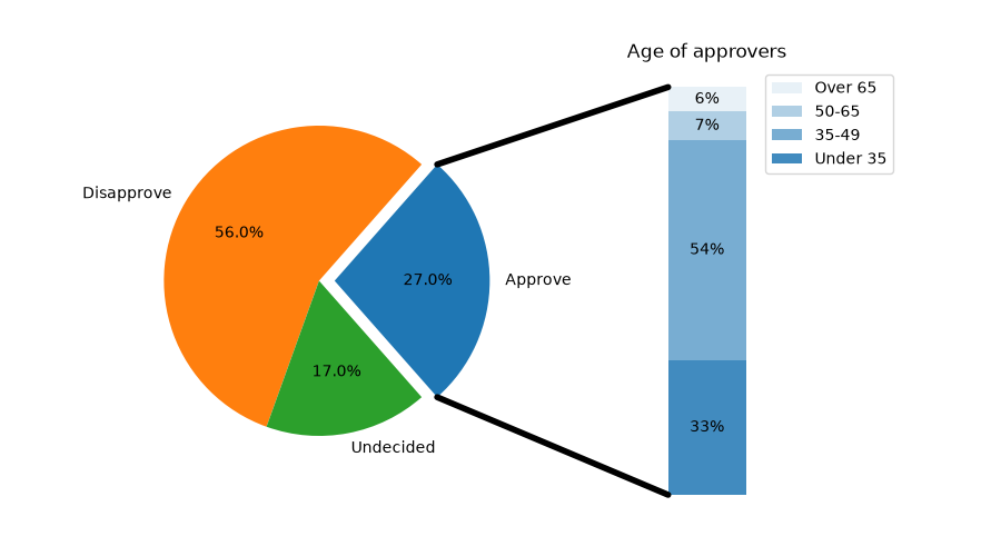
pie_and_polar_charts/nested_pie
=================
Source
"""
=================
Nested pie charts
=================
The following examples show two ways to build a nested pie chart
in Matplotlib. Such charts are often referred to as donut charts.
See also the :doc:`/gallery/specialty_plots/leftventricle_bullseye` example.
"""
import matplotlib.pyplot as plt
import numpy as np
# %%
# The most straightforward way to build a pie chart is to use the
# `~matplotlib.axes.Axes.pie` method.
#
# In this case, pie takes values corresponding to counts in a group.
# We'll first generate some fake data, corresponding to three groups.
# In the inner circle, we'll treat each number as belonging to its
# own group. In the outer circle, we'll plot them as members of their
# original 3 groups.
#
# The effect of the donut shape is achieved by setting a ``width`` to
# the pie's wedges through the *wedgeprops* argument.
fig, ax = plt.subplots()
size = 0.3
vals = np.array([[60., 32.], [37., 40.], [29., 10.]])
tab20c = plt.color_sequences["tab20c"]
outer_colors = [tab20c[i] for i in [0, 4, 8]]
inner_colors = [tab20c[i] for i in [1, 2, 5, 6, 9, 10]]
ax.pie(vals.sum(axis=1), radius=1, colors=outer_colors,
wedgeprops=dict(width=size, edgecolor='w'))
ax.pie(vals.flatten(), radius=1-size, colors=inner_colors,
wedgeprops=dict(width=size, edgecolor='w'))
ax.set(aspect="equal", title='Pie plot with `ax.pie`')
plt.show()
# %%
# However, you can accomplish the same output by using a bar plot on
# Axes with a polar coordinate system. This may give more flexibility on
# the exact design of the plot.
#
# In this case, we need to map x-values of the bar chart onto radians of
# a circle. The cumulative sum of the values are used as the edges
# of the bars.
fig, ax = plt.subplots(subplot_kw=dict(projection="polar"))
size = 0.3
vals = np.array([[60., 32.], [37., 40.], [29., 10.]])
# Normalize vals to 2 pi
valsnorm = vals/np.sum(vals)*2*np.pi
# Obtain the ordinates of the bar edges
valsleft = np.cumsum(np.append(0, valsnorm.flatten()[:-1])).reshape(vals.shape)
cmap = plt.colormaps["tab20c"]
outer_colors = cmap(np.arange(3)*4)
inner_colors = cmap([1, 2, 5, 6, 9, 10])
ax.bar(x=valsleft[:, 0],
width=valsnorm.sum(axis=1), bottom=1-size, height=size,
color=outer_colors, edgecolor='w', linewidth=1, align="edge")
ax.bar(x=valsleft.flatten(),
width=valsnorm.flatten(), bottom=1-2*size, height=size,
color=inner_colors, edgecolor='w', linewidth=1, align="edge")
ax.set(title="Pie plot with `ax.bar` and polar coordinates")
ax.set_axis_off()
plt.show()
# %%
#
# .. admonition:: References
#
# The use of the following functions, methods, classes and modules is shown
# in this example:
#
# - `matplotlib.axes.Axes.pie` / `matplotlib.pyplot.pie`
# - `matplotlib.axes.Axes.bar` / `matplotlib.pyplot.bar`
# - `matplotlib.projections.polar`
# - ``Axes.set`` (`matplotlib.artist.Artist.set`)
# - `matplotlib.axes.Axes.set_axis_off`
#
# .. tags::
#
# plot-type: pie
# level: beginner
# purpose: showcase
pie_and_polar_charts/pie_and_donut_labels
=============================
Source
"""
=============================
A pie and a donut with labels
=============================
Welcome to the Matplotlib bakery. We will create a pie and a donut
chart through the `pie method <matplotlib.axes.Axes.pie>` and
show how to label them with a `legend <matplotlib.axes.Axes.legend>`
as well as with the `pie_label method <matplotlib.axes.Axes.pie>` and
`annotations <matplotlib.axes.Axes.annotate>`.
"""
# %%
# As usual we would start by defining the imports and create a figure with
# subplots.
# Now it's time for the pie. Starting with a pie recipe, we create the data
# and a list of labels from it.
#
# We then create the pie and store the returned `~matplotlib.container.PieContainer`
# object for later.
#
# We can provide the `~matplotlib.container.PieContainer` and a format string to
# the `~matplotlib.axes.Axes.pie_label` method to automatically label each
# ingredient's wedge with its weight in grams and percentages.
#
# The `~.PieContainer` has a list of patches as one of its attributes. Those are
# `matplotlib.patches.Wedge` patches, which can directly be used as the handles
# for a legend. We can use the legend's ``bbox_to_anchor`` argument to position
# the legend outside of the pie. Here we use the axes coordinates ``(1, 0, 0.5,
# 1)`` together with the location ``"center left"``; i.e. the left central
# point of the legend will be at the left central point of the bounding box,
# spanning from ``(1, 0)`` to ``(1.5, 1)`` in axes coordinates.
import matplotlib.pyplot as plt
import numpy as np
fig, ax = plt.subplots(figsize=(6, 3))
recipe = ["375 g flour",
"75 g sugar",
"250 g butter",
"300 g berries"]
data = [int(x.split()[0]) for x in recipe]
ingredients = [x.split()[-1] for x in recipe]
pie = ax.pie(data)
ax.pie_label(pie, '{frac:.1%}\n({absval:d}g)',
textprops=dict(color="w", size=8, weight="bold"))
ax.legend(pie.wedges, ingredients,
title="Ingredients",
loc="center left",
bbox_to_anchor=(1, 0, 0.5, 1))
ax.set_title("Matplotlib bakery: A pie")
plt.show()
# %%
# Now it's time for the donut. Starting with a donut recipe, we transcribe
# the data to numbers (converting 1 egg to 50 g), and directly plot the pie.
# The pie? Wait... it's going to be donut, is it not?
# Well, as we see here, the donut is a pie, having a certain ``width`` set to
# the wedges, which is different from its radius. It's as easy as it gets.
# This is done via the ``wedgeprops`` argument.
#
# We then want to label the wedges via
# `annotations <matplotlib.axes.Axes.annotate>`. We first create some
# dictionaries of common properties, which we can later pass as keyword
# argument. We then iterate over all wedges and for each
#
# * calculate the angle of the wedge's center,
# * from that obtain the coordinates of the point at that angle on the
# circumference,
# * determine the horizontal alignment of the text, depending on which side
# of the circle the point lies,
# * update the connection style with the obtained angle to have the annotation
# arrow point outwards from the donut,
# * finally, create the annotation with all the previously
# determined parameters.
fig, ax = plt.subplots(figsize=(6, 3), subplot_kw=dict(aspect="equal"))
recipe = ["225 g flour",
"90 g sugar",
"1 egg",
"60 g butter",
"100 ml milk",
"1/2 package of yeast"]
data = [225, 90, 50, 60, 100, 5]
pie = ax.pie(data, wedgeprops=dict(width=0.5), startangle=-40)
bbox_props = dict(boxstyle="square,pad=0.3", fc="w", ec="k", lw=0.72)
kw = dict(arrowprops=dict(arrowstyle="-"),
bbox=bbox_props, zorder=0, va="center")
for i, p in enumerate(pie.wedges):
ang = (p.theta2 - p.theta1)/2. + p.theta1
y = np.sin(np.deg2rad(ang))
x = np.cos(np.deg2rad(ang))
horizontalalignment = {-1: "right", 1: "left"}[int(np.sign(x))]
connectionstyle = f"angle,angleA=0,angleB={ang}"
kw["arrowprops"].update({"connectionstyle": connectionstyle})
ax.annotate(recipe[i], xy=(x, y), xytext=(1.35*np.sign(x), 1.4*y),
horizontalalignment=horizontalalignment, **kw)
ax.set_title("Matplotlib bakery: A donut")
plt.show()
# %%
# And here it is, the donut. Note however, that if we were to use this recipe,
# the ingredients would suffice for around 6 donuts - producing one huge
# donut is untested and might result in kitchen errors.
# %%
#
# .. admonition:: References
#
# The use of the following functions, methods, classes and modules is shown
# in this example:
#
# - `matplotlib.axes.Axes.pie` / `matplotlib.pyplot.pie`
# - `matplotlib.axes.Axes.pie_label` / `matplotlib.pyplot.pie_label`
# - `matplotlib.axes.Axes.legend` / `matplotlib.pyplot.legend`
#
# .. tags::
#
# component: label
# component: annotation
# plot-type: pie
# level: beginner
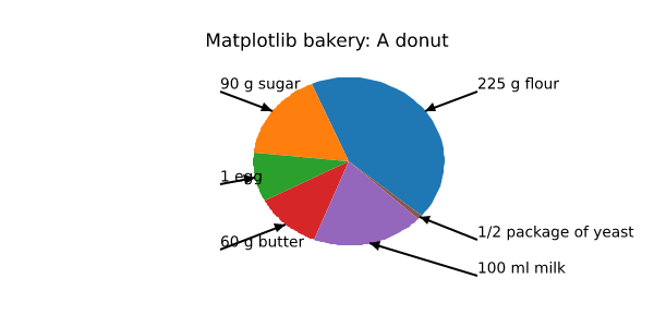
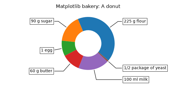
pie_and_polar_charts/pie_features
.. redirect-from:: gallery/pie_and_polar_charts/pie_demo2
Source
"""
.. redirect-from:: gallery/pie_and_polar_charts/pie_demo2
==========
Pie charts
==========
Demo of plotting a pie chart.
This example illustrates various parameters of `~matplotlib.axes.Axes.pie`.
"""
# %%
# Label slices
# ------------
#
# Plot a pie chart of animals and label the slices. To add
# labels, pass a list of labels to the *labels* parameter
import matplotlib.pyplot as plt
labels = 'Frogs', 'Hogs', 'Dogs', 'Logs'
sizes = [15, 30, 45, 10]
fig, ax = plt.subplots()
ax.pie(sizes, labels=labels)
# %%
# Each slice of the pie chart is a `.patches.Wedge` object; therefore in
# addition to the customizations shown here, each wedge can be customized using
# the *wedgeprops* argument, as demonstrated in
# :doc:`/gallery/pie_and_polar_charts/nested_pie`.
#
# Auto-label slices
# -----------------
#
# Pass a function or format string to *autopct* to label slices.
fig, ax = plt.subplots()
ax.pie(sizes, labels=labels, autopct='%1.1f%%')
# %%
# By default, the label values are obtained from the percent size of the slice.
#
# Color slices
# ------------
#
# Pass a list of colors to *colors* to set the color of each slice.
fig, ax = plt.subplots()
ax.pie(sizes, labels=labels,
colors=['olivedrab', 'rosybrown', 'gray', 'saddlebrown'])
# %%
# Hatch slices
# ------------
#
# Pass a list of hatch patterns to *hatch* to set the pattern of each slice.
fig, ax = plt.subplots()
ax.pie(sizes, labels=labels, hatch=['**O', 'oO', 'O.O', '.||.'])
# %%
# Swap label and autopct text positions
# -------------------------------------
# Use the *labeldistance* and *pctdistance* parameters to position the *labels*
# and *autopct* text respectively.
fig, ax = plt.subplots()
ax.pie(sizes, labels=labels, autopct='%1.1f%%',
pctdistance=1.25, labeldistance=.6)
# %%
# *labeldistance* and *pctdistance* are ratios of the radius; therefore they
# vary between ``0`` for the center of the pie and ``1`` for the edge of the
# pie, and can be set to greater than ``1`` to place text outside the pie.
#
# Explode, shade, and rotate slices
# ---------------------------------
#
# In addition to the basic pie chart, this demo shows a few optional features:
#
# * offsetting a slice using *explode*
# * add a drop-shadow using *shadow*
# * custom start angle using *startangle*
#
# This example orders the slices, separates (explodes) them, and rotates them.
explode = (0, 0.1, 0, 0) # only "explode" the 2nd slice (i.e. 'Hogs')
fig, ax = plt.subplots()
ax.pie(sizes, explode=explode, labels=labels, autopct='%1.1f%%',
shadow=True, startangle=90)
plt.show()
# %%
# The default *startangle* is 0, which would start the first slice ("Frogs") on
# the positive x-axis. This example sets ``startangle = 90`` such that all the
# slices are rotated counter-clockwise by 90 degrees, and the frog slice starts
# on the positive y-axis.
#
# Grow or shrink pie
# ------------------
#
# By changing the *radius* parameter, and often the text size for better visual
# appearance, the pie chart can be scaled.
fig, ax = plt.subplots()
ax.pie(sizes, labels=labels, autopct='%.0f%%',
textprops={'size': 'small'}, radius=0.5)
plt.show()
# %%
# Modify shadow
# -------------
#
# The *shadow* parameter may optionally take a dictionary with arguments to
# the `.Shadow` patch. This can be used to modify the default shadow.
fig, ax = plt.subplots()
ax.pie(sizes, explode=explode, labels=labels, autopct='%1.1f%%',
shadow={'ox': -0.04, 'edgecolor': 'none', 'shade': 0.9}, startangle=90)
plt.show()
# %%
# .. admonition:: References
#
# The use of the following functions, methods, classes and modules is shown
# in this example:
#
# - `matplotlib.axes.Axes.pie` / `matplotlib.pyplot.pie`
#
# .. tags::
#
# plot-type: pie
# level: beginner
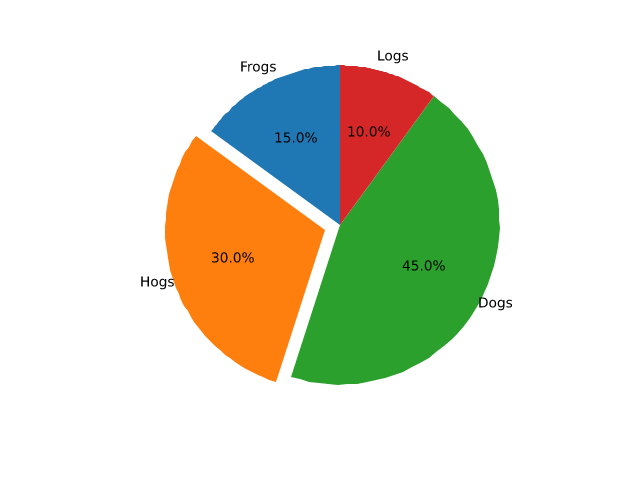
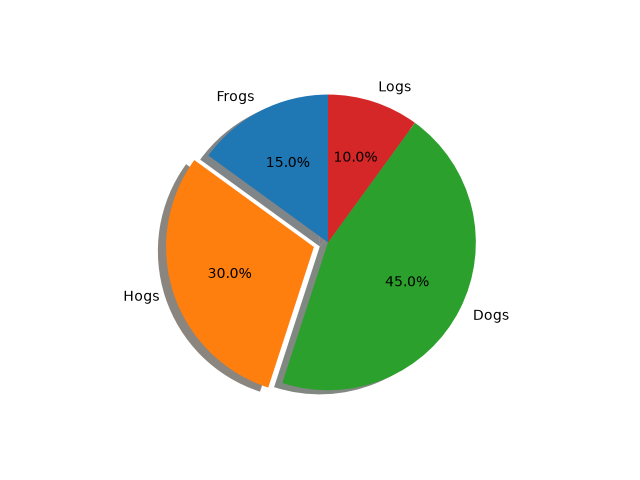
pie_and_polar_charts/pie_label
===================
Source
"""
===================
Labeling pie charts
===================
This example illustrates some features of the `~matplotlib.axes.Axes.pie_label`
method, which adds labels to an existing pie chart created with
`~matplotlib.axes.Axes.pie`.
"""
# %%
# The simplest option is to provide a list of strings to label each slice of the pie.
import matplotlib.pyplot as plt
data = [36, 24, 8, 12]
labels = ['spam', 'eggs', 'bacon', 'sausage']
fig, ax = plt.subplots()
pie = ax.pie(data)
ax.pie_label(pie, labels)
# %%
#
# If you want the labels outside the pie, set a *distance* greater than 1.
# This is the distance from the center of the pie as a fraction of its radius.
fig, ax = plt.subplots()
pie = ax.pie(data)
ax.pie_label(pie, labels, distance=1.1)
# %%
#
# You can also rotate the labels so they are oriented away from the pie center.
fig, ax = plt.subplots()
pie = ax.pie(data)
ax.pie_label(pie, labels, rotate=True)
# %%
#
# Instead of explicit labels, pass a format string to label slices with their values...
fig, ax = plt.subplots()
pie = ax.pie(data)
ax.pie_label(pie, '{absval:.1f}')
# %%
#
# ...or with their percentages...
fig, ax = plt.subplots()
pie = ax.pie(data)
ax.pie_label(pie, '{frac:.1%}')
# %%
#
# ...or both.
fig, ax = plt.subplots()
pie = ax.pie(data)
ax.pie_label(pie, '{absval:d}\n{frac:.1%}')
# %%
#
# Font styling can be configured by passing a dictionary to the *textprops* parameter.
fig, ax = plt.subplots()
pie = ax.pie(data)
ax.pie_label(pie, labels, textprops={'fontsize': 'large', 'color': 'white'})
# %%
#
# `~matplotlib.axes.Axes.pie_label` can be called repeatedly to add multiple sets
# of labels.
# sphinx_gallery_thumbnail_number = -1
fig, ax = plt.subplots()
pie = ax.pie(data)
ax.pie_label(pie, labels, distance=1.1)
ax.pie_label(pie, '{frac:.1%}', distance=0.7)
ax.pie_label(pie, '{absval:d}', distance=0.4)
plt.show()
# %%
# .. admonition:: References
#
# The use of the following functions, methods, classes and modules is shown
# in this example:
#
# - `matplotlib.axes.Axes.pie` / `matplotlib.pyplot.pie`
# - `matplotlib.axes.Axes.pie_label` / `matplotlib.pyplot.pie_label`
#
# .. tags::
#
# plot-type: pie
# level: beginner
pie_and_polar_charts/polar_bar
=======================
Source
""" ======================= Bar chart on polar axis ======================= Demo of bar plot on a polar axis. """ import matplotlib.pyplot as plt import numpy as np # Fixing random state for reproducibility np.random.seed(19680801) # Compute pie slices N = 20 theta = np.linspace(0.0, 2 * np.pi, N, endpoint=False) radii = 10 * np.random.rand(N) width = np.pi / 4 * np.random.rand(N) colors = plt.colormaps["viridis"](radii / 10.) ax = plt.subplot(projection='polar') ax.bar(theta, radii, width=width, bottom=0.0, color=colors, alpha=0.5) plt.show() # %% # # .. admonition:: References # # The use of the following functions, methods, classes and modules is shown # in this example: # # - `matplotlib.axes.Axes.bar` / `matplotlib.pyplot.bar` # - `matplotlib.projections.polar` # # .. tags:: # # plot-type: pie # plot-type: bar # level: beginner # purpose: showcase
pie_and_polar_charts/polar_demo
==========
Source
"""
==========
Polar plot
==========
Demo of a line plot on a polar axis.
The second plot shows the same data, but with the radial axis starting at r=1
and the angular axis starting at 0 degrees and ending at 225 degrees. Setting
the origin of the radial axis to 0 allows the radial ticks to be placed at the
same location as the first plot.
"""
import matplotlib.pyplot as plt
import numpy as np
r = np.arange(0, 2, 0.01)
theta = 2 * np.pi * r
fig, axs = plt.subplots(2, 1, figsize=(5, 8), subplot_kw={'projection': 'polar'},
layout='constrained')
ax = axs[0]
ax.plot(theta, r)
ax.set_rmax(2)
ax.set_rticks([0.5, 1, 1.5, 2]) # Fewer radial ticks
ax.set_rlabel_position(-22.5) # Move radial labels away from plotted line
ax.grid(True)
ax.set_title("A line plot on a polar axis", va='bottom')
ax = axs[1]
ax.plot(theta, r)
ax.set_rmax(2)
ax.set_rmin(1) # Change the radial axis to only go from 1 to 2
ax.set_rorigin(0) # Set the origin of the radial axis to 0
ax.set_thetamin(0)
ax.set_thetamax(225)
ax.set_rticks([1, 1.5, 2]) # Fewer radial ticks
ax.set_rlabel_position(-22.5) # Move radial labels away from plotted line
ax.grid(True)
ax.set_title("Same plot, but with reduced axis limits", va='bottom')
plt.show()
# %%
#
# .. admonition:: References
#
# The use of the following functions, methods, classes and modules is shown
# in this example:
#
# - `matplotlib.axes.Axes.plot` / `matplotlib.pyplot.plot`
# - `matplotlib.projections.polar`
# - `matplotlib.projections.polar.PolarAxes`
# - `matplotlib.projections.polar.PolarAxes.set_rticks`
# - `matplotlib.projections.polar.PolarAxes.set_rmin`
# - `matplotlib.projections.polar.PolarAxes.set_rorigin`
# - `matplotlib.projections.polar.PolarAxes.set_rmax`
# - `matplotlib.projections.polar.PolarAxes.set_rlabel_position`
#
# .. tags::
#
# plot-type: polar
# level: beginner
pie_and_polar_charts/polar_error_caps
=================================
Source
"""
=================================
Error bar rendering on polar axis
=================================
Demo of error bar plot in polar coordinates.
Theta error bars are curved lines ended with caps oriented towards the
center.
Radius error bars are straight lines oriented towards center with
perpendicular caps.
"""
import matplotlib.pyplot as plt
import numpy as np
theta = np.arange(0, 2 * np.pi, np.pi / 4)
r = theta / np.pi / 2 + 0.5
fig = plt.figure(figsize=(10, 10))
ax = fig.add_subplot(projection='polar')
ax.errorbar(theta, r, xerr=0.25, yerr=0.1, capsize=7, fmt="o", c="seagreen")
ax.set_title("Pretty polar error bars")
plt.show()
# %%
# Please acknowledge that large theta error bars will be overlapping.
# This may reduce readability of the output plot. See example figure below:
fig = plt.figure(figsize=(10, 10))
ax = fig.add_subplot(projection='polar')
ax.errorbar(theta, r, xerr=5.25, yerr=0.1, capsize=7, fmt="o", c="darkred")
ax.set_title("Overlapping theta error bars")
plt.show()
# %%
# On the other hand, large radius error bars will never overlap, they just
# lead to unwanted scale in the data, reducing the displayed range.
fig = plt.figure(figsize=(10, 10))
ax = fig.add_subplot(projection='polar')
ax.errorbar(theta, r, xerr=0.25, yerr=10.1, capsize=7, fmt="o", c="orangered")
ax.set_title("Large radius error bars")
plt.show()
# %%
#
# .. admonition:: References
#
# The use of the following functions, methods, classes and modules is shown
# in this example:
#
# - `matplotlib.axes.Axes.errorbar` / `matplotlib.pyplot.errorbar`
# - `matplotlib.projections.polar`
#
# .. tags::
#
# component: error
# plot-type: errorbar
# plot-type: polar
# level: beginner
pie_and_polar_charts/polar_legend
============
Source
"""
============
Polar legend
============
Using a legend on a polar-axis plot.
"""
import matplotlib.pyplot as plt
import numpy as np
fig = plt.figure()
ax = fig.add_subplot(projection="polar", facecolor="lightgoldenrodyellow")
r = np.linspace(0, 3, 301)
theta = 2 * np.pi * r
ax.plot(theta, r, color="tab:orange", lw=3, label="a line")
ax.plot(0.5 * theta, r, color="tab:blue", ls="--", lw=3, label="another line")
ax.tick_params(grid_color="palegoldenrod")
# For polar Axes, it may be useful to move the legend slightly away from the
# Axes center, to avoid overlap between the legend and the Axes. The following
# snippet places the legend's lower left corner just outside the polar Axes
# at an angle of 67.5 degrees in polar coordinates.
angle = np.deg2rad(67.5)
ax.legend(loc="lower left",
bbox_to_anchor=(.5 + np.cos(angle)/2, .5 + np.sin(angle)/2))
plt.show()
# %%
#
# .. admonition:: References
#
# The use of the following functions, methods, classes and modules is shown
# in this example:
#
# - `matplotlib.axes.Axes.plot` / `matplotlib.pyplot.plot`
# - `matplotlib.axes.Axes.legend` / `matplotlib.pyplot.legend`
# - `matplotlib.projections.polar`
# - `matplotlib.projections.polar.PolarAxes`
#
# .. tags::
#
# component: legend
# plot-type: polar
# level: beginner
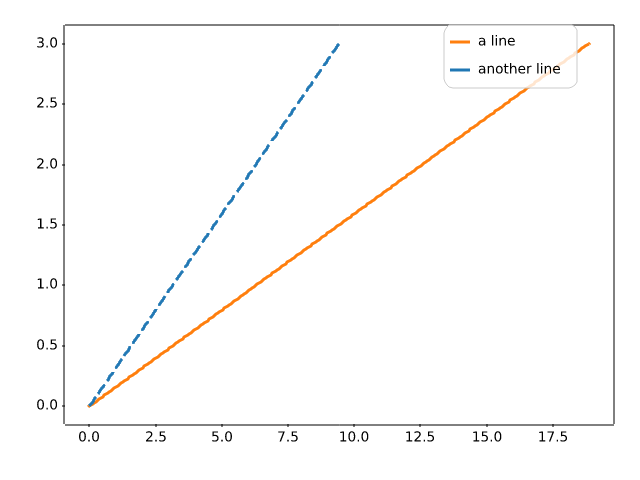
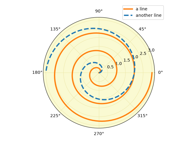
pie_and_polar_charts/polar_scatter
==========================
Source
"""
==========================
Scatter plot on polar axis
==========================
Size increases radially in this example and color increases with angle
(just to verify the symbols are being scattered correctly).
"""
import matplotlib.pyplot as plt
import numpy as np
# Fixing random state for reproducibility
np.random.seed(19680801)
# Compute areas and colors
N = 150
r = 2 * np.random.rand(N)
theta = 2 * np.pi * np.random.rand(N)
area = 200 * r**2
colors = theta
fig = plt.figure()
ax = fig.add_subplot(projection='polar')
c = ax.scatter(theta, r, c=colors, s=area, cmap='hsv', alpha=0.75)
# %%
# Scatter plot on polar axis, with offset origin
# ----------------------------------------------
#
# The main difference with the previous plot is the configuration of the origin
# radius, producing an annulus. Additionally, the theta zero location is set to
# rotate the plot.
fig = plt.figure()
ax = fig.add_subplot(projection='polar')
c = ax.scatter(theta, r, c=colors, s=area, cmap='hsv', alpha=0.75)
ax.set_rorigin(-2.5)
ax.set_theta_zero_location('W', offset=10)
# %%
# Scatter plot on polar axis confined to a sector
# -----------------------------------------------
#
# The main difference with the previous plots is the configuration of the
# theta start and end limits, producing a sector instead of a full circle.
fig = plt.figure()
ax = fig.add_subplot(projection='polar')
c = ax.scatter(theta, r, c=colors, s=area, cmap='hsv', alpha=0.75)
ax.set_thetamin(45)
ax.set_thetamax(135)
plt.show()
# %%
#
# .. admonition:: References
#
# The use of the following functions, methods, classes and modules is shown
# in this example:
#
# - `matplotlib.axes.Axes.scatter` / `matplotlib.pyplot.scatter`
# - `matplotlib.projections.polar`
# - `matplotlib.projections.polar.PolarAxes.set_rorigin`
# - `matplotlib.projections.polar.PolarAxes.set_theta_zero_location`
# - `matplotlib.projections.polar.PolarAxes.set_thetamin`
# - `matplotlib.projections.polar.PolarAxes.set_thetamax`
#
# .. tags::
#
# plot-type: polar
# plot-type: scatter
# level: beginner
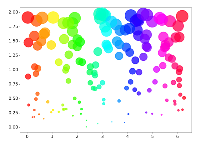
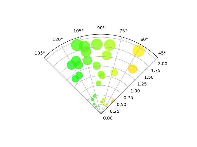
pyplots/pyplot_simple
==========
Source
"""
==========
Basic plot
==========
A basic plot using the :ref:`pyplot_interface`.
- `~.pyplot.plot` plots the data y versus x as lines and/or markers.
- `~.pyplot.title`, `~.pyplot.xlabel` and `~.pyplot.ylabel` set the title,
x-axis label and y-axis label.
- `~.pyplot.show` displays the plot.
.. redirect-from:: /gallery/pyplots/fig_axes_labels_simple
.. redirect-from:: /gallery/pyplots/pyplot_formatstr
.. redirect-from:: /gallery/pyplots/pyplot_text
"""
import matplotlib.pyplot as plt
import numpy as np
x = np.arange(0.0, 2.0, 0.01)
y = np.sin(2 * np.pi * x)
plt.plot(x, y)
plt.title("A basic plot using pyplot")
plt.xlabel('Time [s]')
plt.ylabel('Voltage [mV]')
plt.show()
# %%
#
# .. admonition:: References
#
# The use of the following functions, methods, classes and modules is shown
# in this example:
#
# - `matplotlib.pyplot.plot`
# - `matplotlib.pyplot.title`
# - `matplotlib.pyplot.ylabel`
# - `matplotlib.pyplot.ylabel`
# - `matplotlib.pyplot.show`
pyplots/pyplot_two_subplots
=========================
Source
"""
=========================
Two subplots using pyplot
=========================
A typical pyplot usage pattern is to create subplots incrementally through
`~.pyplot.subplot`.
The three-digit number passed to `~.pyplot.subplot` specifies the position of
the subplot in the grid of subplots. ``211`` means "in a grid of 2 rows and 1 column,
create this subplot in the 1st position". ``212`` likewise means "in a grid of 2
rows and 1 column, create this subplot in the 2nd position".
After calling ``subplot()`` all following pyplot commands will modify that subplot
until a new subplot is created.
.. redirect-from:: /gallery/pyplots/pyplot_three
"""
import matplotlib.pyplot as plt
import numpy as np
def f(t):
return np.exp(-t) * np.cos(2*np.pi*t)
t1 = np.arange(0.0, 5.0, 0.1)
t2 = np.arange(0.0, 5.0, 0.02)
plt.figure()
plt.subplot(211)
plt.plot(t1, f(t1), color='tab:blue', marker='o')
plt.plot(t2, f(t2), color='black')
plt.title("Subplot 1")
plt.subplot(212)
plt.plot(t2, np.cos(2*np.pi*t2), color='tab:orange', linestyle='--')
plt.title("Subplot 2")
plt.show()
# %%
#
# .. admonition:: References
#
# The use of the following functions, methods, classes and modules is shown
# in this example:
#
# - `matplotlib.pyplot.figure`
# - `matplotlib.pyplot.subplot`
scales/asinh_demo
===========
Source
"""
===========
Asinh scale
===========
Illustration of the `asinh <.scale.AsinhScale>` axis scaling,
which uses the transformation
.. math::
a \\rightarrow a_0 \\sinh^{-1} (a / a_0)
For coordinate values close to zero (i.e. much smaller than
the "linear width" :math:`a_0`), this leaves values essentially unchanged:
.. math::
a \\rightarrow a + \\mathcal{O}(a^3)
but for larger values (i.e. :math:`|a| \\gg a_0`, this is asymptotically
.. math::
a \\rightarrow a_0 \\, \\mathrm{sgn}(a) \\ln |a| + \\mathcal{O}(1)
As with the `symlog <.scale.SymmetricalLogScale>` scaling,
this allows one to plot quantities
that cover a very wide dynamic range that includes both positive
and negative values. However, ``symlog`` involves a transformation
that has discontinuities in its gradient because it is built
from *separate* linear and logarithmic transformations.
The ``asinh`` scaling uses a transformation that is smooth
for all (finite) values, which is both mathematically cleaner
and reduces visual artifacts associated with an abrupt
transition between linear and logarithmic regions of the plot.
.. note::
`.scale.AsinhScale` is experimental, and the API may change.
See `~.scale.AsinhScale`, `~.scale.SymmetricalLogScale`.
"""
import matplotlib.pyplot as plt
import numpy as np
# Prepare sample values for variations on y=x graph:
x = np.linspace(-3, 6, 500)
# %%
# Compare "symlog" and "asinh" behaviour on sample y=x graph,
# where there is a discontinuous gradient in "symlog" near y=2:
fig1 = plt.figure()
ax0, ax1 = fig1.subplots(1, 2, sharex=True)
ax0.plot(x, x)
ax0.set_yscale('symlog')
ax0.grid()
ax0.set_title('symlog')
ax1.plot(x, x)
ax1.set_yscale('asinh')
ax1.grid()
ax1.set_title('asinh')
# %%
# Compare "asinh" graphs with different scale parameter "linear_width":
fig2 = plt.figure(layout='constrained')
axs = fig2.subplots(1, 3, sharex=True)
for ax, (a0, base) in zip(axs, ((0.2, 2), (1.0, 0), (5.0, 10))):
ax.set_title(f'linear_width={a0:.3g}')
ax.plot(x, x, label='y=x')
ax.plot(x, 10*x, label='y=10x')
ax.plot(x, 100*x, label='y=100x')
ax.set_yscale('asinh', linear_width=a0, base=base)
ax.grid()
ax.legend(loc='best', fontsize='small')
# %%
# Compare "symlog" and "asinh" scalings
# on 2D Cauchy-distributed random numbers,
# where one may be able to see more subtle artifacts near y=2
# due to the gradient-discontinuity in "symlog":
fig3 = plt.figure()
ax = fig3.subplots(1, 1)
r = 3 * np.tan(np.random.uniform(-np.pi / 2.02, np.pi / 2.02,
size=(5000,)))
th = np.random.uniform(0, 2*np.pi, size=r.shape)
ax.scatter(r * np.cos(th), r * np.sin(th), s=4, alpha=0.5)
ax.set_xscale('asinh')
ax.set_yscale('symlog')
ax.set_xlabel('asinh')
ax.set_ylabel('symlog')
ax.set_title('2D Cauchy random deviates')
ax.set_xlim(-50, 50)
ax.set_ylim(-50, 50)
ax.grid()
plt.show()
# %%
#
# .. admonition:: References
#
# - `matplotlib.scale.AsinhScale`
# - `matplotlib.ticker.AsinhLocator`
# - `matplotlib.scale.SymmetricalLogScale`
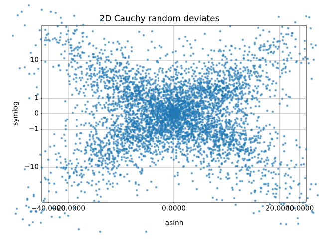
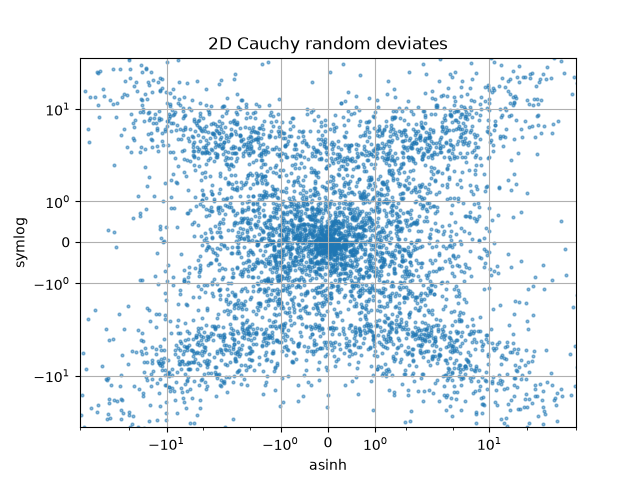
scales/aspect_loglog
=============
Source
"""
=============
Loglog aspect
=============
"""
import matplotlib.pyplot as plt
fig, (ax1, ax2) = plt.subplots(1, 2)
ax1.set_xscale("log")
ax1.set_yscale("log")
ax1.set_xlim(1e1, 1e3)
ax1.set_ylim(1e2, 1e3)
ax1.set_aspect(1)
ax1.set_title("adjustable = box")
ax2.set_xscale("log")
ax2.set_yscale("log")
ax2.set_adjustable("datalim")
ax2.plot([1, 3, 10], [1, 9, 100], "o-")
ax2.set_xlim(1e-1, 1e2)
ax2.set_ylim(1e-1, 1e3)
ax2.set_aspect(1)
ax2.set_title("adjustable = datalim")
plt.show()
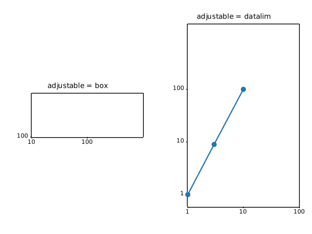
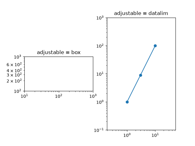
scales/custom_scale
.. _custom_scale:
Source
"""
.. _custom_scale:
============
Custom scale
============
Custom scales can be created in two ways
#. For simple cases, use `~.scale.FuncScale` and the ``'function'`` option of
`~.Axes.set_xscale` and `~.Axes.set_yscale`. See the last example in
:doc:`/gallery/scales/scales`.
#. Create a custom scale class such as the one in this example, which implements
the scaling use for latitude data in a Mercator Projection. This more complicated
approach is useful when
* You are making special use of the `.Transform` class, such as the special
handling of values beyond the threshold in ``MercatorLatitudeTransform``
below.
* You want to override the default locators and formatters for the axis
(``set_default_locators_and_formatters`` below).
* You want to limit the range of the axis (``limit_range_for_scale`` below).
"""
import numpy as np
from numpy import ma
from matplotlib import scale as mscale
from matplotlib import transforms as mtransforms
from matplotlib.ticker import FixedLocator, FuncFormatter
class MercatorLatitudeScale(mscale.ScaleBase):
"""
Scales data in range -pi/2 to pi/2 (-90 to 90 degrees) using
the system used to scale latitudes in a Mercator__ projection.
The scale function:
ln(tan(y) + sec(y))
The inverse scale function:
atan(sinh(y))
Since the Mercator scale tends to infinity at +/- 90 degrees,
there is user-defined threshold, above and below which nothing
will be plotted. This defaults to +/- 85 degrees.
__ https://en.wikipedia.org/wiki/Mercator_projection
"""
# The scale class must have a member ``name`` that defines the string used
# to select the scale. For example, ``ax.set_yscale("mercator")`` would be
# used to select this scale.
name = 'mercator'
def __init__(self, axis, *, thresh=np.deg2rad(85), **kwargs):
"""
Any keyword arguments passed to ``set_xscale`` and ``set_yscale`` will
be passed along to the scale's constructor.
thresh: The degree above which to crop the data.
"""
super().__init__(axis)
if thresh >= np.pi / 2:
raise ValueError("thresh must be less than pi/2")
self.thresh = thresh
def get_transform(self):
"""
Override this method to return a new instance that does the
actual transformation of the data.
The MercatorLatitudeTransform class is defined below as a
nested class of this one.
"""
return self.MercatorLatitudeTransform(self.thresh)
def set_default_locators_and_formatters(self, axis):
"""
Override to set up the locators and formatters to use with the
scale. This is only required if the scale requires custom
locators and formatters. Writing custom locators and
formatters is rather outside the scope of this example, but
there are many helpful examples in :mod:`.ticker`.
In our case, the Mercator example uses a fixed locator from -90 to 90
degrees and a custom formatter to convert the radians to degrees and
put a degree symbol after the value.
"""
fmt = FuncFormatter(
lambda x, pos=None: f"{np.degrees(x):.0f}\N{DEGREE SIGN}")
axis.set(major_locator=FixedLocator(np.radians(range(-90, 90, 10))),
major_formatter=fmt, minor_formatter=fmt)
def limit_range_for_scale(self, vmin, vmax, minpos):
"""
Override to limit the bounds of the axis to the domain of the
transform. In the case of Mercator, the bounds should be
limited to the threshold that was passed in. Unlike the
autoscaling provided by the tick locators, this range limiting
will always be adhered to, whether the axis range is set
manually, determined automatically or changed through panning
and zooming.
"""
return max(vmin, -self.thresh), min(vmax, self.thresh)
class MercatorLatitudeTransform(mtransforms.Transform):
# There are two value members that must be defined.
# ``input_dims`` and ``output_dims`` specify number of input
# dimensions and output dimensions to the transformation.
# These are used by the transformation framework to do some
# error checking and prevent incompatible transformations from
# being connected together. When defining transforms for a
# scale, which are, by definition, separable and have only one
# dimension, these members should always be set to 1.
input_dims = output_dims = 1
def __init__(self, thresh):
mtransforms.Transform.__init__(self)
self.thresh = thresh
def transform_non_affine(self, a):
"""
This transform takes a numpy array and returns a transformed copy.
Since the range of the Mercator scale is limited by the
user-specified threshold, the input array must be masked to
contain only valid values. Matplotlib will handle masked arrays
and remove the out-of-range data from the plot. However, the
returned array *must* have the same shape as the input array, since
these values need to remain synchronized with values in the other
dimension.
"""
masked = ma.masked_where((a < -self.thresh) | (a > self.thresh), a)
if masked.mask.any():
return ma.log(np.abs(ma.tan(masked) + 1 / ma.cos(masked)))
else:
return np.log(np.abs(np.tan(a) + 1 / np.cos(a)))
def inverted(self):
"""
Override this method so Matplotlib knows how to get the
inverse transform for this transform.
"""
return MercatorLatitudeScale.InvertedMercatorLatitudeTransform(
self.thresh)
class InvertedMercatorLatitudeTransform(mtransforms.Transform):
input_dims = output_dims = 1
def __init__(self, thresh):
mtransforms.Transform.__init__(self)
self.thresh = thresh
def transform_non_affine(self, a):
return np.arctan(np.sinh(a))
def inverted(self):
return MercatorLatitudeScale.MercatorLatitudeTransform(self.thresh)
# Now that the Scale class has been defined, it must be registered so
# that Matplotlib can find it.
mscale.register_scale(MercatorLatitudeScale)
if __name__ == '__main__':
import matplotlib.pyplot as plt
t = np.arange(-180.0, 180.0, 0.1)
s = np.radians(t)/2.
plt.plot(t, s, '-', lw=2)
plt.yscale('mercator')
plt.xlabel('Longitude')
plt.ylabel('Latitude')
plt.title('Mercator projection')
plt.grid(True)
plt.show()
AttributeError: module 'matplotvite' has no attribute 'scale'
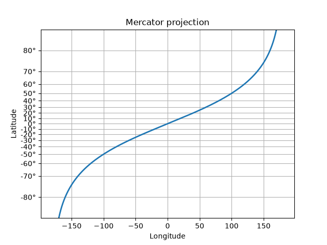
scales/log_demo
=========
Source
"""
=========
Log scale
=========
Examples of plots with logarithmic axes.
You can set the x/y axes to be logarithmic by passing "log" to `~.Axes.set_xscale` /
`~.Axes.set_yscale`.
Convenience functions ``semilogx``, ``semilogy``, and ``loglog``
----------------------------------------------------------------
Since plotting data on semi-logarithmic or double-logarithmic scales is very common,
the functions `~.Axes.semilogx`, `~.Axes.semilogy`, and `~.Axes.loglog` are shortcuts
for setting the scale and plotting data; e.g. ``ax.semilogx(x, y)`` is equivalent to
``ax.set_xscale('log'); ax.plot(x, y)``.
"""
import matplotlib.pyplot as plt
import numpy as np
fig, (ax1, ax2, ax3) = plt.subplots(1, 3, layout='constrained', figsize=(7, 7/3))
# log x axis
t = np.arange(0.01, 10.0, 0.01)
ax1.semilogx(t, np.sin(2 * np.pi * t))
ax1.set(title='semilogx')
ax1.grid()
ax1.grid(which="minor", color="0.9")
# log y axis
x = np.arange(4)
ax2.semilogy(4*x, 10**x, 'o--')
ax2.set(title='semilogy')
ax2.grid()
ax2.grid(which="minor", color="0.9")
# log x and y axis
x = np.array([1, 10, 100, 1000])
ax3.loglog(x, 5 * x, 'o--')
ax3.set(title='loglog')
ax3.grid()
ax3.grid(which="minor", color="0.9")
# %%
# Logarithms with other bases
# ---------------------------
# By default, the log scale is to the base 10. One can change this via the *base*
# parameter.
fig, ax = plt.subplots()
ax.bar(["L1 cache", "L2 cache", "L3 cache", "RAM", "SSD"],
[32, 1_000, 32_000, 16_000_000, 512_000_000])
ax.set_yscale('log', base=2)
ax.set_yticks([1, 2**10, 2**20, 2**30], labels=['kB', 'MB', 'GB', 'TB'])
ax.set_title("Typical memory sizes")
ax.yaxis.grid()
# %%
# Dealing with negative values
# ----------------------------
# Non-positive values cannot be displayed on a log scale. The scale has two options
# to handle these. Either mask the values so that they are ignored, or clip them
# to a small positive value. Which one is more suited depends on the type of the
# data and the visualization.
#
# The following example contains errorbars going negative. If we mask these values,
# the bar vanishes, which is not desirable. In contrast, clipping makes the value
# small positive (but well below the used scale) so that the error bar is drawn
# to the edge of the Axes.
x = np.linspace(0.0, 2.0, 10)
y = 10**x
yerr = 1.75 + 0.75*y
fig, (ax1, ax2) = plt.subplots(1, 2, layout="constrained", figsize=(6, 3))
fig.suptitle("errorbars going negative")
ax1.set_yscale("log", nonpositive='mask')
ax1.set_title('nonpositive="mask"')
ax1.errorbar(x, y, yerr=yerr, fmt='o', capsize=5)
ax2.set_yscale("log", nonpositive='clip')
ax2.set_title('nonpositive="clip"')
ax2.errorbar(x, y, yerr=yerr, fmt='o', capsize=5)
plt.show()
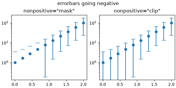
scales/logit_demo
===========
Source
"""
===========
Logit scale
===========
Examples of plots with logit axes.
This example visualises how ``set_yscale("logit")`` works on probability plots
by generating three distributions: normal, laplacian, and cauchy in one plot.
The advantage of logit scale is that it effectively spreads out values close to 0 and 1.
In a linear scale plot, probability values near 0 and 1 appear compressed,
making it difficult to see differences in those regions.
In a logit scale plot, the transformation expands these regions,
making the graph cleaner and easier to compare across different probability values.
This makes the logit scale especially useful when visalising probabilities in logistic
regression, classification models, and cumulative distribution functions.
"""
import math
import matplotlib.pyplot as plt
import numpy as np
xmax = 10
x = np.linspace(-xmax, xmax, 10000)
cdf_norm = [math.erf(w / np.sqrt(2)) / 2 + 1 / 2 for w in x]
cdf_laplacian = np.where(x < 0, 1 / 2 * np.exp(x), 1 - 1 / 2 * np.exp(-x))
cdf_cauchy = np.arctan(x) / np.pi + 1 / 2
fig, axs = plt.subplots(nrows=3, ncols=2, figsize=(6.4, 8.5))
# Common part, for the example, we will do the same plots on all graphs
for i in range(3):
for j in range(2):
axs[i, j].plot(x, cdf_norm, label=r"$\mathcal{N}$")
axs[i, j].plot(x, cdf_laplacian, label=r"$\mathcal{L}$")
axs[i, j].plot(x, cdf_cauchy, label="Cauchy")
axs[i, j].legend()
axs[i, j].grid()
# First line, logitscale, with standard notation
axs[0, 0].set(title="logit scale")
axs[0, 0].set_yscale("logit")
axs[0, 0].set_ylim(1e-5, 1 - 1e-5)
axs[0, 1].set(title="logit scale")
axs[0, 1].set_yscale("logit")
axs[0, 1].set_xlim(0, xmax)
axs[0, 1].set_ylim(0.8, 1 - 5e-3)
# Second line, logitscale, with survival notation (with `use_overline`), and
# other format display 1/2
axs[1, 0].set(title="logit scale")
axs[1, 0].set_yscale("logit", one_half="1/2", use_overline=True)
axs[1, 0].set_ylim(1e-5, 1 - 1e-5)
axs[1, 1].set(title="logit scale")
axs[1, 1].set_yscale("logit", one_half="1/2", use_overline=True)
axs[1, 1].set_xlim(0, xmax)
axs[1, 1].set_ylim(0.8, 1 - 5e-3)
# Third line, linear scale
axs[2, 0].set(title="linear scale")
axs[2, 0].set_ylim(0, 1)
axs[2, 1].set(title="linear scale")
axs[2, 1].set_xlim(0, xmax)
axs[2, 1].set_ylim(0.8, 1)
fig.tight_layout()
plt.show()
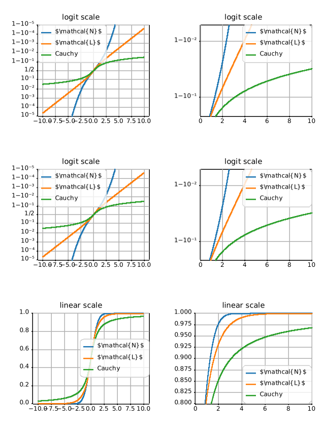
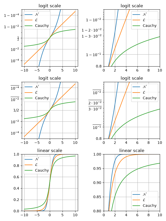
scales/power_norm
========================
Source
"""
========================
Exploring normalizations
========================
Various normalization on a multivariate normal distribution.
"""
import matplotlib.pyplot as plt
import numpy as np
from numpy.random import multivariate_normal
import matplotlib.colors as mcolors
# Fixing random state for reproducibility.
np.random.seed(19680801)
data = np.vstack([
multivariate_normal([10, 10], [[3, 2], [2, 3]], size=100000),
multivariate_normal([30, 20], [[3, 1], [1, 3]], size=1000)
])
gammas = [0.8, 0.5, 0.3]
fig, axs = plt.subplots(nrows=2, ncols=2)
axs[0, 0].set_title('Linear normalization')
axs[0, 0].hist2d(data[:, 0], data[:, 1], bins=100)
for ax, gamma in zip(axs.flat[1:], gammas):
ax.set_title(r'Power law $(\gamma=%1.1f)$' % gamma)
ax.hist2d(data[:, 0], data[:, 1], bins=100, norm=mcolors.PowerNorm(gamma))
fig.tight_layout()
plt.show()
# %%
#
# .. admonition:: References
#
# The use of the following functions, methods, classes and modules is shown
# in this example:
#
# - `matplotlib.colors`
# - `matplotlib.colors.PowerNorm`
# - `matplotlib.axes.Axes.hist2d`
# - `matplotlib.pyplot.hist2d`
NameError: name 'multivariate_normal' is not defined
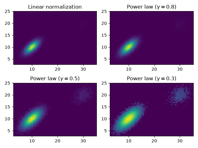
scales/scales
===============
Source
"""
===============
Scales overview
===============
Illustrate the scale transformations applied to axes, e.g. log, symlog, logit.
See `matplotlib.scale` for a full list of built-in scales,
:doc:`/gallery/scales/custom_scale` for how to create your own scale, and
:doc:`/gallery/mplot3d/scales3d` for using scales on 3D axes.
"""
import matplotlib.pyplot as plt
import numpy as np
x = np.arange(400)
y = np.linspace(0.002, 1, 400)
fig, axs = plt.subplots(3, 2, figsize=(6, 8), layout='constrained')
axs[0, 0].plot(x, y)
axs[0, 0].set_yscale('linear')
axs[0, 0].set_title('linear')
axs[0, 0].grid(True)
axs[0, 1].plot(x, y)
axs[0, 1].set_yscale('log')
axs[0, 1].set_title('log')
axs[0, 1].grid(True)
axs[1, 0].plot(x, y - y.mean())
axs[1, 0].set_yscale('symlog', linthresh=0.02)
axs[1, 0].set_title('symlog')
axs[1, 0].grid(True)
axs[1, 1].plot(x, y)
axs[1, 1].set_yscale('logit')
axs[1, 1].set_title('logit')
axs[1, 1].grid(True)
axs[2, 0].plot(x, y - y.mean())
axs[2, 0].set_yscale('asinh', linear_width=0.01)
axs[2, 0].set_title('asinh')
axs[2, 0].grid(True)
# Function x**(1/2)
def forward(x):
return x**(1/2)
def inverse(x):
return x**2
axs[2, 1].plot(x, y)
axs[2, 1].set_yscale('function', functions=(forward, inverse))
axs[2, 1].set_title('function: $x^{1/2}$')
axs[2, 1].grid(True)
axs[2, 1].set_yticks(np.arange(0, 1.2, 0.2))
plt.show()
# %%
#
# .. admonition:: References
#
# The use of the following functions, methods, classes and modules is shown
# in this example:
#
# - `matplotlib.axes.Axes.set_xscale`
# - `matplotlib.axes.Axes.set_yscale`
# - `matplotlib.scale.LinearScale`
# - `matplotlib.scale.LogScale`
# - `matplotlib.scale.SymmetricalLogScale`
# - `matplotlib.scale.LogitScale`
# - `matplotlib.scale.FuncScale`
NotImplementedError: unsupported y scale: 'function'
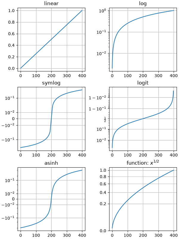
scales/symlog_demo
============
Source
"""
============
Symlog scale
============
The symmetric logarithmic scale is an extension of the logarithmic scale that
also covers negative values. As with the logarithmic scale, it is particularly
useful for numerical data that spans a broad range of values, especially when there
are significant differences between the magnitudes of the numbers involved.
Example use of symlog (symmetric log) axis scaling.
"""
import matplotlib.pyplot as plt
import numpy as np
dt = 0.01
x = np.arange(-50.0, 50.0, dt)
y = np.arange(0, 100.0, dt)
fig, (ax0, ax1, ax2) = plt.subplots(nrows=3)
ax0.plot(x, y)
ax0.set_xscale('symlog')
ax0.set_ylabel('symlogx')
ax0.grid()
ax0.xaxis.grid(which='minor') # minor grid on too
ax1.plot(y, x)
ax1.set_yscale('symlog')
ax1.set_ylabel('symlogy')
ax2.plot(x, np.sin(x / 3.0))
ax2.set_xscale('symlog')
ax2.set_yscale('symlog', linthresh=0.015)
ax2.grid()
ax2.set_ylabel('symlog both')
fig.tight_layout()
plt.show()
# %%
# Linear threshold
# ----------------
# Since each decade on a logarithmic scale covers the same amount of visual space
# and there are infinitely many decades between a given number and zero, the symlog
# scale must deviate from logarithmic mapping in a small range
# *(-linthresh, linthresh)*, so that the range is mapped to a finite visual space.
def format_axes(ax, title=None):
"""A helper function to better visualize properties of the symlog scale."""
ax.xaxis.get_minor_locator().set_params(subs=[2, 3, 4, 5, 6, 7, 8, 9])
ax.grid()
ax.xaxis.grid(which='minor') # minor grid on too
linthresh = ax.xaxis.get_transform().linthresh
linscale = ax.xaxis.get_transform().linscale
ax.axvspan(-linthresh, linthresh, color='0.9')
if title:
ax.set_title(title.format(linthresh=linthresh, linscale=linscale))
x = np.linspace(-60, 60, 201)
y = np.linspace(0, 100.0, 201)
fig, (ax1, ax2) = plt.subplots(nrows=2, layout="constrained")
ax1.plot(x, y)
ax1.set_xscale('symlog', linthresh=1)
format_axes(ax1, title='Linear region: linthresh={linthresh}')
ax2.plot(x, y)
ax2.set_xscale('symlog', linthresh=5)
format_axes(ax2, title='Linear region: linthresh={linthresh}')
# %%
# Generally, *linthresh* should be chosen so that no or only a few
# data points are in the linear region. As a rule of thumb,
# :math:`linthresh \approx \mathrm{min} |x|`.
#
#
# Linear scale
# ------------
# Additionally, the *linscale* parameter determines how much visual space should be
# used for the linear range. More precisely, it defines the ratio of visual space
# of the region (0, linthresh) relative to one decade.
fig, (ax1, ax2) = plt.subplots(nrows=2, layout="constrained")
ax1.plot(x, y)
ax1.set_xscale('symlog', linthresh=1)
format_axes(ax1, title='Linear region: linthresh={linthresh}, linscale={linscale}')
ax2.plot(x, y)
ax2.set_xscale('symlog', linthresh=1, linscale=0.1)
format_axes(ax2, title='Linear region: linthresh={linthresh}, linscale={linscale}')
# %%
# The suitable value for linscale depends on the dynamic range of data. As most data
# will be outside the linear region, you typically the linear region only to cover
# a small fraction of the visual area.
#
# Limitations and alternatives
# ----------------------------
# The coordinate transform used by ``symlog`` has a discontinuous gradient at the
# transition between its linear and logarithmic regions. Depending on data and
# scaling, this will be more or less obvious in the plot.
fig, ax = plt.subplots()
ax.plot(x, y)
ax.set_xscale('symlog', linscale=0.05)
format_axes(ax, title="Discontinuous gradient at linear/log transition")
# %%
# The ``asinh`` axis scale is an alternative transformation that supports a wide
# dynamic range with a smooth gradient and thus may avoid such visual artifacts.
# See :doc:`/gallery/scales/asinh_demo`.
#
#
# .. admonition:: References
#
# - `matplotlib.scale.SymmetricalLogScale`
# - `matplotlib.ticker.SymmetricalLogLocator`
# - `matplotlib.scale.AsinhScale`
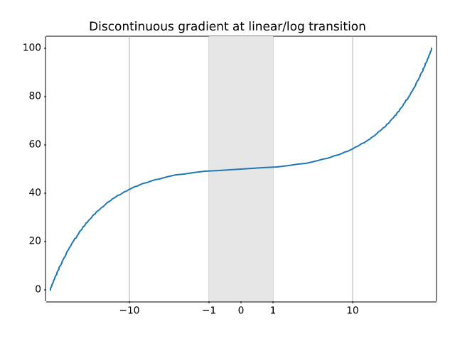
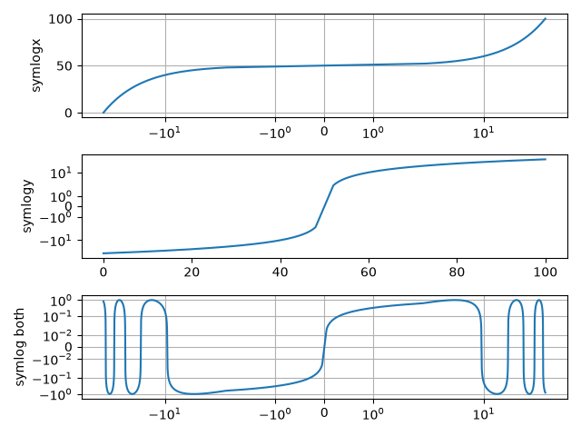
shapes_and_collections/arrow_guide
===========
Source
"""
===========
Arrow guide
===========
Adding arrow patches to plots.
Arrows are often used to annotate plots. This tutorial shows how to plot arrows
that behave differently when the data limits on a plot are changed. In general,
points on a plot can either be fixed in "data space" or "display space".
Something plotted in data space moves when the data limits are altered - an
example would be the points in a scatter plot. Something plotted in display
space stays static when data limits are altered - an example would be a
figure title or the axis labels.
Arrows consist of a head (and possibly a tail) and a stem drawn between a
start point and end point, called 'anchor points' from now on.
Here we show three use cases for plotting arrows, depending on whether the
head or anchor points need to be fixed in data or display space:
1. Head shape fixed in display space, anchor points fixed in data space
2. Head shape and anchor points fixed in display space
3. Entire patch fixed in data space
Below each use case is presented in turn.
.. redirect-from:: /gallery/text_labels_and_annotations/arrow_simple_demo
"""
import matplotlib.pyplot as plt
import matplotlib.patches as mpatches
x_tail = 0.1
y_tail = 0.5
x_head = 0.9
y_head = 0.8
dx = x_head - x_tail
dy = y_head - y_tail
# %%
# Head shape fixed in display space and anchor points fixed in data space
# -----------------------------------------------------------------------
#
# This is useful if you are annotating a plot, and don't want the arrow
# to change shape or position if you pan or scale the plot.
#
# In this case we use `.patches.FancyArrowPatch`.
#
# Note that when the axis limits are changed, the arrow shape stays the same,
# but the anchor points move.
fig, axs = plt.subplots(nrows=2)
arrow = mpatches.FancyArrowPatch((x_tail, y_tail), (x_head, y_head),
mutation_scale=100)
axs[0].add_patch(arrow)
arrow = mpatches.FancyArrowPatch((x_tail, y_tail), (x_head, y_head),
mutation_scale=100)
axs[1].add_patch(arrow)
axs[1].set(xlim=(0, 2), ylim=(0, 2))
# %%
# Head shape and anchor points fixed in display space
# ---------------------------------------------------
#
# This is useful if you are annotating a plot, and don't want the arrow to
# change shape or position if you pan or scale the plot.
#
# In this case we use `.patches.FancyArrowPatch`, and pass the keyword argument
# ``transform=ax.transAxes`` where ``ax`` is the Axes we are adding the patch
# to.
#
# Note that when the axis limits are changed, the arrow shape and location
# stay the same.
fig, axs = plt.subplots(nrows=2)
arrow = mpatches.FancyArrowPatch((x_tail, y_tail), (x_head, y_head),
mutation_scale=100,
transform=axs[0].transAxes)
axs[0].add_patch(arrow)
arrow = mpatches.FancyArrowPatch((x_tail, y_tail), (x_head, y_head),
mutation_scale=100,
transform=axs[1].transAxes)
axs[1].add_patch(arrow)
axs[1].set(xlim=(0, 2), ylim=(0, 2))
# %%
# Head shape and anchor points fixed in data space
# ------------------------------------------------
#
# In this case we use `.patches.Arrow`, or `.patches.FancyArrow` (the latter is
# in orange).
#
# Note that when the axis limits are changed, the arrow shape and location
# change.
#
# `.FancyArrow`'s API is relatively awkward, and requires in particular passing
# ``length_includes_head=True`` so that the arrow *tip* is ``(dx, dy)`` away
# from the arrow start. It is only included in this reference because it is
# the arrow class returned by `.Axes.arrow` (in green).
fig, axs = plt.subplots(nrows=2)
arrow = mpatches.Arrow(x_tail, y_tail, dx, dy)
axs[0].add_patch(arrow)
arrow = mpatches.FancyArrow(x_tail, y_tail - .4, dx, dy,
width=.1, length_includes_head=True, color="C1")
axs[0].add_patch(arrow)
axs[0].arrow(x_tail + 1, y_tail - .4, dx, dy,
width=.1, length_includes_head=True, color="C2")
arrow = mpatches.Arrow(x_tail, y_tail, dx, dy)
axs[1].add_patch(arrow)
arrow = mpatches.FancyArrow(x_tail, y_tail - .4, dx, dy,
width=.1, length_includes_head=True, color="C1")
axs[1].add_patch(arrow)
axs[1].arrow(x_tail + 1, y_tail - .4, dx, dy,
width=.1, length_includes_head=True, color="C2")
axs[1].set(xlim=(0, 2), ylim=(0, 2))
# %%
plt.show()
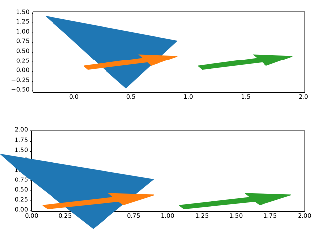
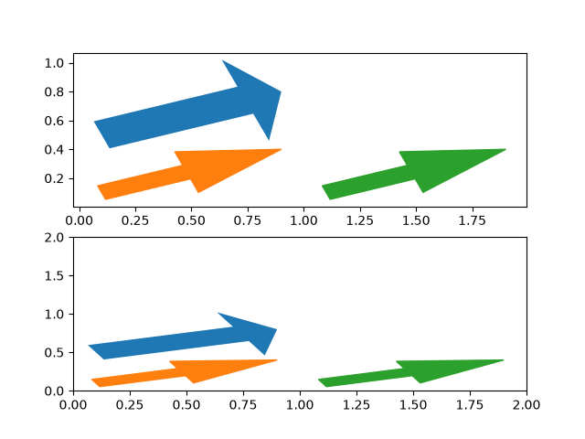
shapes_and_collections/artist_reference
.. _artist_reference:
Source
"""
.. _artist_reference:
================================
Reference for Matplotlib artists
================================
This example displays several of Matplotlib's graphics primitives (artists).
A full list of artists is documented at :ref:`the artist API <artist-api>`.
See also :doc:`/gallery/shapes_and_collections/patch_collection`, which groups
all artists into a single `.PatchCollection` instead.
Copyright (c) 2010, Bartosz Telenczuk
BSD License
"""
import matplotlib.pyplot as plt
import matplotlib as mpl
import matplotlib.lines as mlines
import matplotlib.patches as mpatches
import matplotlib.path as mpath
# Prepare the data for the PathPatch below.
Path = mpath.Path
codes, verts = zip(*[
(Path.MOVETO, [0.018, -0.11]),
(Path.CURVE4, [-0.031, -0.051]),
(Path.CURVE4, [-0.115, 0.073]),
(Path.CURVE4, [-0.03, 0.073]),
(Path.LINETO, [-0.011, 0.039]),
(Path.CURVE4, [0.043, 0.121]),
(Path.CURVE4, [0.075, -0.005]),
(Path.CURVE4, [0.035, -0.027]),
(Path.CLOSEPOLY, [0.018, -0.11])])
artists = [
mpatches.Circle((0, 0), 0.1, ec="none"),
mpatches.Rectangle((-0.025, -0.05), 0.05, 0.1, ec="none"),
mpatches.Wedge((0, 0), 0.1, 30, 270, ec="none"),
mpatches.RegularPolygon((0, 0), 5, radius=0.1),
mpatches.Ellipse((0, 0), 0.2, 0.1),
mpatches.Arrow(-0.05, -0.05, 0.1, 0.1, width=0.1),
mpatches.PathPatch(mpath.Path(verts, codes), ec="none"),
mpatches.FancyBboxPatch((-0.025, -0.05), 0.05, 0.1, ec="none",
boxstyle=mpatches.BoxStyle("Round", pad=0.02)),
mlines.Line2D([-0.06, 0.0, 0.1], [0.05, -0.05, 0.05], lw=5),
]
axs = plt.figure(figsize=(6, 6), layout="constrained").subplots(3, 3)
for i, (ax, artist) in enumerate(zip(axs.flat, artists)):
artist.set(color=mpl.colormaps["hsv"](i / len(artists)))
ax.add_artist(artist)
ax.set(title=type(artist).__name__,
aspect=1, xlim=(-.2, .2), ylim=(-.2, .2))
ax.set_axis_off()
plt.show()
# %%
#
# .. admonition:: References
#
# The use of the following functions, methods, classes and modules is shown
# in this example:
#
# - `matplotlib.path`
# - `matplotlib.path.Path`
# - `matplotlib.lines`
# - `matplotlib.lines.Line2D`
# - `matplotlib.patches`
# - `matplotlib.patches.Circle`
# - `matplotlib.patches.Ellipse`
# - `matplotlib.patches.Wedge`
# - `matplotlib.patches.Rectangle`
# - `matplotlib.patches.Arrow`
# - `matplotlib.patches.PathPatch`
# - `matplotlib.patches.FancyBboxPatch`
# - `matplotlib.patches.RegularPolygon`
# - `matplotlib.axes.Axes.add_artist`
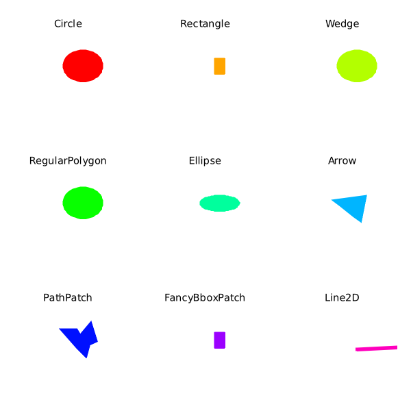
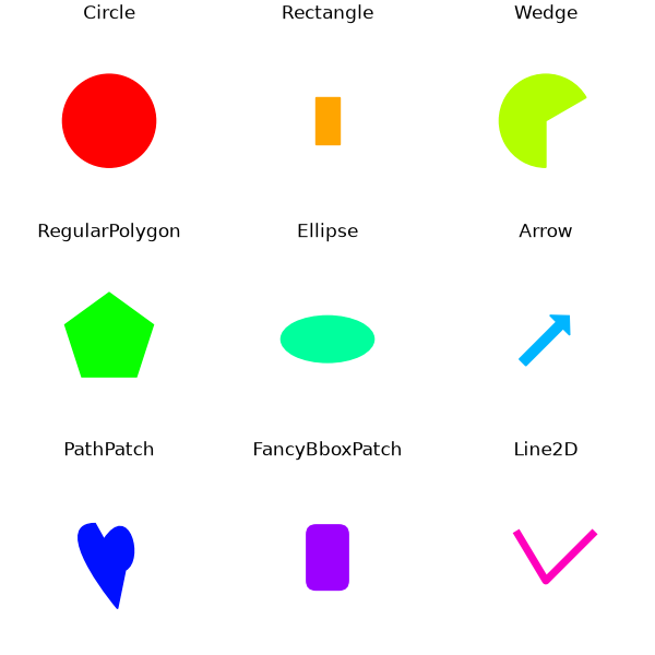
shapes_and_collections/collections
=====================================
Source
"""
=====================================
Line, Poly and RegularPoly Collection
=====================================
For the first two subplots, we will use spirals. Their size will be set in
plot units, not data units. Their positions will be set in data units by using
the *offsets* and *offset_transform* keyword arguments of the `.LineCollection`
and `.PolyCollection`.
The third subplot will make regular polygons, with the same
type of scaling and positioning as in the first two.
The last subplot illustrates the use of ``offsets=(xo, yo)``,
that is, a single tuple instead of a list of tuples, to generate
successively offset curves, with the offset given in data
units. This behavior is available only for the LineCollection.
"""
import matplotlib.pyplot as plt
import numpy as np
from matplotlib import collections, transforms
nverts = 50
npts = 100
# Make some spirals
r = np.arange(nverts)
theta = np.linspace(0, 2*np.pi, nverts)
xx = r * np.sin(theta)
yy = r * np.cos(theta)
spiral = np.column_stack([xx, yy])
# Fixing random state for reproducibility
rs = np.random.RandomState(19680801)
# Make some offsets
xyo = rs.randn(npts, 2)
# Make a list of colors from the default color cycle.
colors = plt.rcParams['axes.prop_cycle'].by_key()['color']
fig, ((ax1, ax2), (ax3, ax4)) = plt.subplots(2, 2)
fig.subplots_adjust(top=0.92, left=0.07, right=0.97,
hspace=0.3, wspace=0.3)
col = collections.LineCollection(
[spiral], offsets=xyo, offset_transform=ax1.transData, color=colors)
# transform the line segments such that their size is given in points
trans = fig.dpi_scale_trans + transforms.Affine2D().scale(1.0/72.0)
col.set_transform(trans) # the points to pixels transform
ax1.add_collection(col)
ax1.set_title('LineCollection using offsets')
# The same data as above, but fill the curves.
col = collections.PolyCollection(
[spiral], offsets=xyo, offset_transform=ax2.transData, color=colors)
trans = transforms.Affine2D().scale(fig.dpi/72.0)
col.set_transform(trans) # the points to pixels transform
ax2.add_collection(col)
ax2.set_title('PolyCollection using offsets')
# 7-sided regular polygons
col = collections.RegularPolyCollection(
7, sizes=np.abs(xx) * 10.0, offsets=xyo, offset_transform=ax3.transData,
color=colors)
trans = transforms.Affine2D().scale(fig.dpi / 72.0)
col.set_transform(trans) # the points to pixels transform
ax3.add_collection(col)
ax3.set_title('RegularPolyCollection using offsets')
# Simulate a series of ocean current profiles, successively
# offset by 0.1 m/s so that they form what is sometimes called
# a "waterfall" plot or a "stagger" plot.
nverts = 60
ncurves = 20
offs = (0.1, 0.0)
yy = np.linspace(0, 2*np.pi, nverts)
ym = np.max(yy)
xx = (0.2 + (ym - yy) / ym) ** 2 * np.cos(yy - 0.4) * 0.5
segs = []
for i in range(ncurves):
xxx = xx + 0.02*rs.randn(nverts)
curve = np.column_stack([xxx, yy * 100])
segs.append(curve)
col = collections.LineCollection(segs, offsets=offs, color=colors)
ax4.add_collection(col)
ax4.set_title('Successive data offsets')
ax4.set_xlabel('Zonal velocity component (m/s)')
ax4.set_ylabel('Depth (m)')
ax4.invert_yaxis() # so that depth increases downward
plt.show()
# %%
#
# .. admonition:: References
#
# The use of the following functions, methods, classes and modules is shown
# in this example:
#
# - `matplotlib.figure.Figure`
# - `matplotlib.collections`
# - `matplotlib.collections.LineCollection`
# - `matplotlib.collections.RegularPolyCollection`
# - `matplotlib.axes.Axes.add_collection`
# - `matplotlib.transforms.Affine2D`
# - `matplotlib.transforms.Affine2D.scale`
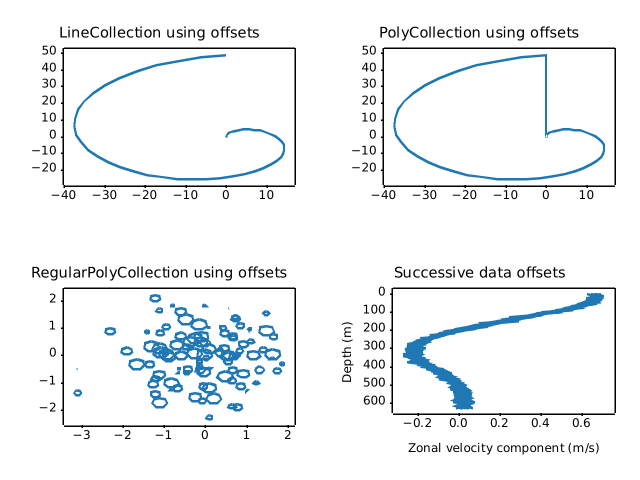
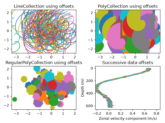
shapes_and_collections/compound_path
=============
Source
"""
=============
Compound path
=============
Make a compound path -- in this case two simple polygons, a rectangle
and a triangle. Use ``CLOSEPOLY`` and ``MOVETO`` for the different parts of
the compound path
"""
import matplotlib.pyplot as plt
from matplotlib.patches import PathPatch
from matplotlib.path import Path
vertices = []
codes = []
codes = [Path.MOVETO] + [Path.LINETO]*3 + [Path.CLOSEPOLY]
vertices = [(1, 1), (1, 2), (2, 2), (2, 1), (0, 0)]
codes += [Path.MOVETO] + [Path.LINETO]*2 + [Path.CLOSEPOLY]
vertices += [(4, 4), (5, 5), (5, 4), (0, 0)]
path = Path(vertices, codes)
pathpatch = PathPatch(path, facecolor='none', edgecolor='green')
fig, ax = plt.subplots()
ax.add_patch(pathpatch)
ax.set_title('A compound path')
ax.autoscale_view()
plt.show()
# %%
#
# .. admonition:: References
#
# The use of the following functions, methods, classes and modules is shown
# in this example:
#
# - `matplotlib.path`
# - `matplotlib.path.Path`
# - `matplotlib.patches`
# - `matplotlib.patches.PathPatch`
# - `matplotlib.axes.Axes.add_patch`
# - `matplotlib.axes.Axes.autoscale_view`
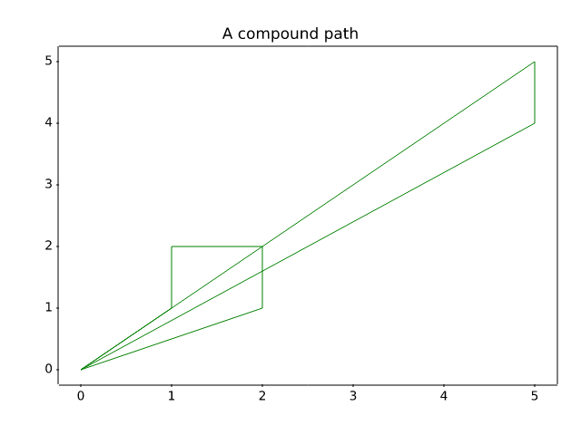
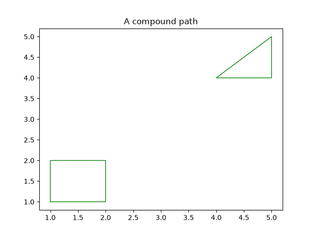
shapes_and_collections/dolphin
========
Source
"""
========
Dolphins
========
This example shows how to draw, and manipulate shapes given vertices
and nodes using the `~.path.Path`, `~.patches.PathPatch` and
`~matplotlib.transforms` classes.
"""
import matplotlib.pyplot as plt
import numpy as np
from matplotlib.patches import Circle, PathPatch
from matplotlib.path import Path
from matplotlib.transforms import Affine2D
# Fixing random state for reproducibility
np.random.seed(19680801)
r = np.random.rand(50)
t = np.random.rand(50) * np.pi * 2.0
x = r * np.cos(t)
y = r * np.sin(t)
fig, ax = plt.subplots(figsize=(6, 6))
circle = Circle((0, 0), 1, facecolor='none',
edgecolor=(0, 0.8, 0.8), linewidth=3, alpha=0.5)
ax.add_patch(circle)
im = plt.imshow(np.random.random((100, 100)),
origin='lower', cmap="winter",
interpolation='spline36',
extent=(-1, 1, -1, 1))
im.set_clip_path(circle)
plt.plot(x, y, 'o', color=(0.9, 0.9, 1.0), alpha=0.8)
# Dolphin from OpenClipart library by Andy Fitzsimon (Public Domain).
dolphin = """
M -0.59739425,160.18173 C -0.62740401,160.18885 -0.57867129,160.11183
-0.57867129,160.11183 C -0.57867129,160.11183 -0.5438361,159.89315
-0.39514638,159.81496 C -0.24645668,159.73678 -0.18316813,159.71981
-0.18316813,159.71981 C -0.18316813,159.71981 -0.10322971,159.58124
-0.057804323,159.58725 C -0.029723983,159.58913 -0.061841603,159.60356
-0.071265813,159.62815 C -0.080250183,159.65325 -0.082918513,159.70554
-0.061841203,159.71248 C -0.040763903,159.7194 -0.0066711426,159.71091
0.077336307,159.73612 C 0.16879567,159.76377 0.28380306,159.86448
0.31516668,159.91533 C 0.3465303,159.96618 0.5011127,160.1771
0.5011127,160.1771 C 0.63668998,160.19238 0.67763022,160.31259
0.66556395,160.32668 C 0.65339985,160.34212 0.66350443,160.33642
0.64907098,160.33088 C 0.63463742,160.32533 0.61309688,160.297
0.5789627,160.29339 C 0.54348657,160.28968 0.52329693,160.27674
0.50728856,160.27737 C 0.49060916,160.27795 0.48965803,160.31565
0.46114204,160.33673 C 0.43329696,160.35786 0.4570711,160.39871
0.43309565,160.40685 C 0.4105108,160.41442 0.39416631,160.33027
0.3954995,160.2935 C 0.39683269,160.25672 0.43807996,160.21522
0.44567915,160.19734 C 0.45327833,160.17946 0.27946869,159.9424
-0.061852613,159.99845 C -0.083965233,160.0427 -0.26176109,160.06683
-0.26176109,160.06683 C -0.30127962,160.07028 -0.21167141,160.09731
-0.24649368,160.1011 C -0.32642366,160.11569 -0.34521187,160.06895
-0.40622293,160.0819 C -0.467234,160.09485 -0.56738444,160.17461
-0.59739425,160.18173
"""
vertices = []
codes = []
parts = dolphin.split()
i = 0
code_map = {
'M': Path.MOVETO,
'C': Path.CURVE4,
'L': Path.LINETO,
}
while i < len(parts):
path_code = code_map[parts[i]]
npoints = Path.NUM_VERTICES_FOR_CODE[path_code]
codes.extend([path_code] * npoints)
vertices.extend([[*map(float, y.split(','))]
for y in parts[i + 1:][:npoints]])
i += npoints + 1
vertices = np.array(vertices)
vertices[:, 1] -= 160
dolphin_path = Path(vertices, codes)
dolphin_patch = PathPatch(dolphin_path, facecolor=(0.6, 0.6, 0.6),
edgecolor=(0.0, 0.0, 0.0))
ax.add_patch(dolphin_patch)
vertices = Affine2D().rotate_deg(60).transform(vertices)
dolphin_path2 = Path(vertices, codes)
dolphin_patch2 = PathPatch(dolphin_path2, facecolor=(0.5, 0.5, 0.5),
edgecolor=(0.0, 0.0, 0.0))
ax.add_patch(dolphin_patch2)
plt.show()
# %%
#
# .. admonition:: References
#
# The use of the following functions, methods, classes and modules is shown
# in this example:
#
# - `matplotlib.path`
# - `matplotlib.path.Path`
# - `matplotlib.patches`
# - `matplotlib.patches.PathPatch`
# - `matplotlib.patches.Circle`
# - `matplotlib.axes.Axes.add_patch`
# - `matplotlib.transforms`
# - `matplotlib.transforms.Affine2D`
# - `matplotlib.transforms.Affine2D.rotate_deg`
#
# .. tags::
#
# component: patch
# styling: shape
# purpose: fun
shapes_and_collections/donut
=============
Source
r"""
=============
Mmh Donuts!!!
=============
Draw donuts (miam!) using `~.path.Path`\s and `~.patches.PathPatch`\es.
This example shows the effect of the path's orientations in a compound path.
"""
import matplotlib.pyplot as plt
import numpy as np
import matplotlib.patches as mpatches
import matplotlib.path as mpath
def wise(v):
return {+1: "CCW", -1: "CW"}[v]
def make_circle(r):
t = np.arange(0, np.pi * 2.0, 0.01)
x = r * np.cos(t)
y = r * np.sin(t)
return np.column_stack((x, y))
fig, ax = plt.subplots()
inside_vertices = make_circle(0.5)
outside_vertices = make_circle(1.0)
codes = np.full(len(inside_vertices), mpath.Path.LINETO)
codes[0] = mpath.Path.MOVETO
for i, (inside, outside) in enumerate(((1, 1), (1, -1), (-1, 1), (-1, -1))):
# Concatenate the inside and outside subpaths together, changing their
# order as needed
vertices = np.concatenate((outside_vertices[::outside],
inside_vertices[::inside]))
# Shift the path
vertices += (i * 2.5, 0)
# The codes will be all "LINETO" commands, except for "MOVETO"s at the
# beginning of each subpath
all_codes = np.concatenate((codes, codes))
# Create the Path object
path = mpath.Path(vertices, all_codes)
# And plot it
patch = mpatches.PathPatch(path, facecolor='#885500', edgecolor='black')
ax.add_patch(patch)
ax.annotate(f"Outside {wise(outside)},\nInside {wise(inside)}",
(i * 2.5, -1.5), va="top", ha="center")
ax.set(xlim=(-2, 10), ylim=(-3, 2), aspect=1, title="Mmm, donuts!")
plt.show()
# %%
#
# .. admonition:: References
#
# The use of the following functions, methods, classes and modules is shown
# in this example:
#
# - `matplotlib.path`
# - `matplotlib.path.Path`
# - `matplotlib.patches`
# - `matplotlib.patches.PathPatch`
# - `matplotlib.patches.Circle`
# - `matplotlib.axes.Axes.add_patch`
# - `matplotlib.axes.Axes.annotate`
# - `matplotlib.axes.Axes.set_aspect`
# - `matplotlib.axes.Axes.set_xlim`
# - `matplotlib.axes.Axes.set_ylim`
# - `matplotlib.axes.Axes.set_title`
#
# .. tags::
#
# component: patch
# styling: shape
# purpose: fun
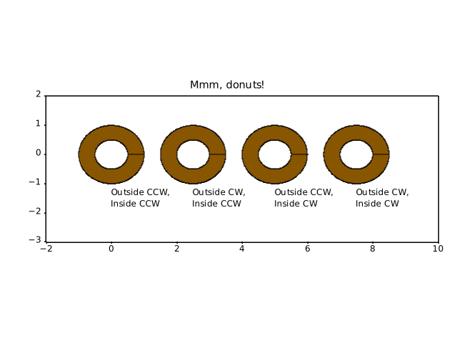
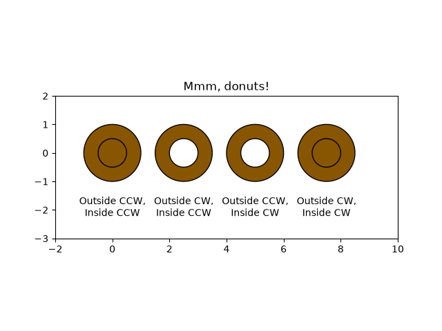
shapes_and_collections/ellipse_arrow
===================================
Source
"""
===================================
Ellipse with orientation arrow demo
===================================
This demo shows how to draw an ellipse with
an orientation arrow (clockwise or counterclockwise).
Compare this to the :doc:`Ellipse collection example
</gallery/shapes_and_collections/ellipse_collection>`.
"""
import matplotlib.pyplot as plt
from matplotlib.markers import MarkerStyle
from matplotlib.patches import Ellipse
from matplotlib.transforms import Affine2D
# Create a figure and axis
fig, ax = plt.subplots(subplot_kw={"aspect": "equal"})
ellipse = Ellipse(
xy=(2, 4),
width=30,
height=20,
angle=35,
facecolor="none",
edgecolor="b"
)
ax.add_patch(ellipse)
# Plot an arrow marker at the end point of minor axis
vertices = ellipse.get_co_vertices()
t = Affine2D().rotate_deg(ellipse.angle)
ax.plot(
vertices[0][0],
vertices[0][1],
color="b",
marker=MarkerStyle(">", "full", t),
markersize=10
)
# Note: To reverse the orientation arrow, switch the marker type from > to <.
plt.show()
# %%
#
# .. admonition:: References
#
# The use of the following functions, methods, classes and modules is shown
# in this example:
#
# - `matplotlib.patches`
# - `matplotlib.patches.Ellipse`
shapes_and_collections/ellipse_collection
==================
Source
"""
==================
Ellipse Collection
==================
Drawing a collection of ellipses. While this would equally be possible using
a `~.collections.EllipseCollection` or `~.collections.PathCollection`, the use
of an `~.collections.EllipseCollection` allows for much shorter code.
"""
import matplotlib.pyplot as plt
import numpy as np
from matplotlib.collections import EllipseCollection
x = np.arange(10)
y = np.arange(15)
X, Y = np.meshgrid(x, y)
XY = np.column_stack((X.ravel(), Y.ravel()))
ww = X / 10.0
hh = Y / 15.0
aa = X * 9
fig, ax = plt.subplots()
ec = EllipseCollection(ww, hh, aa, units='x', offsets=XY,
offset_transform=ax.transData)
ec.set_array((X + Y).ravel())
ax.add_collection(ec)
ax.set_xlabel('X')
ax.set_ylabel('y')
cbar = plt.colorbar(ec)
cbar.set_label('X+Y')
plt.show()
# %%
#
# .. admonition:: References
#
# The use of the following functions, methods, classes and modules is shown
# in this example:
#
# - `matplotlib.collections`
# - `matplotlib.collections.EllipseCollection`
# - `matplotlib.axes.Axes.add_collection`
# - `matplotlib.cm.ScalarMappable.set_array`
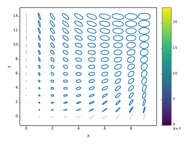
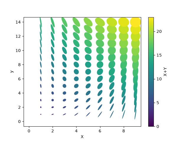
shapes_and_collections/ellipse_demo
============
Source
"""
============
Ellipse Demo
============
Draw many ellipses. Here individual ellipses are drawn. Compare this
to the :doc:`Ellipse collection example
</gallery/shapes_and_collections/ellipse_collection>`.
"""
import matplotlib.pyplot as plt
import numpy as np
from matplotlib.patches import Ellipse
# Fixing random state for reproducibility
np.random.seed(19680801)
NUM = 250
ells = [Ellipse(xy=np.random.rand(2) * 10,
width=np.random.rand(), height=np.random.rand(),
angle=np.random.rand() * 360)
for i in range(NUM)]
fig, ax = plt.subplots()
ax.set(xlim=(0, 10), ylim=(0, 10), aspect="equal")
for e in ells:
ax.add_artist(e)
e.set_clip_box(ax.bbox)
e.set_alpha(np.random.rand())
e.set_facecolor(np.random.rand(3))
plt.show()
# %%
# ===============
# Ellipse Rotated
# ===============
#
# Draw many ellipses with different angles.
#
angle_step = 45 # degrees
angles = np.arange(0, 180, angle_step)
fig, ax = plt.subplots()
ax.set(xlim=(-2.2, 2.2), ylim=(-2.2, 2.2), aspect="equal")
for angle in angles:
ellipse = Ellipse((0, 0), 4, 2, angle=angle, alpha=0.1)
ax.add_artist(ellipse)
plt.show()
# %%
#
# .. admonition:: References
#
# The use of the following functions, methods, classes and modules is shown
# in this example:
#
# - `matplotlib.patches`
# - `matplotlib.patches.Ellipse`
# - `matplotlib.axes.Axes.add_artist`
# - `matplotlib.artist.Artist.set_clip_box`
# - `matplotlib.artist.Artist.set_alpha`
# - `matplotlib.patches.Patch.set_facecolor`
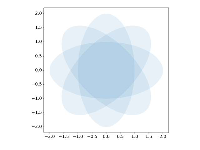
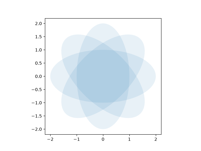
shapes_and_collections/fancybox_demo
===================
Source
"""
===================
Drawing fancy boxes
===================
The following examples show how to plot boxes (`.FancyBboxPatch`) with different
visual properties.
"""
import inspect
import matplotlib.pyplot as plt
import matplotlib.patches as mpatch
from matplotlib.patches import FancyBboxPatch
import matplotlib.transforms as mtransforms
# %%
# Box styles
# ----------
# `.FancyBboxPatch` supports different `.BoxStyle`\s. Note that `~.Axes.text`
# allows to draw a box around the text by adding the ``bbox`` parameter. Therefore,
# you don't see explicit `.FancyBboxPatch` and `.BoxStyle` calls in the following
# example.
styles = mpatch.BoxStyle.get_styles()
ncol = 2
nrow = (len(styles) + 1) // ncol
axs = (plt.figure(figsize=(3 * ncol, 1 + nrow))
.add_gridspec(1 + nrow, ncol, wspace=.5).subplots())
for ax in axs.flat:
ax.set_axis_off()
for ax in axs[0, :]:
ax.text(.2, .5, "boxstyle",
transform=ax.transAxes, size="large", color="tab:blue",
horizontalalignment="right", verticalalignment="center")
ax.text(.4, .5, "default parameters",
transform=ax.transAxes,
horizontalalignment="left", verticalalignment="center")
for ax, (stylename, stylecls) in zip(axs[1:, :].T.flat, styles.items()):
ax.text(.2, .5, stylename, bbox=dict(boxstyle=stylename, fc="w", ec="k"),
transform=ax.transAxes, size="large", color="tab:blue",
horizontalalignment="right", verticalalignment="center")
ax.text(.4, .5, str(inspect.signature(stylecls))[1:-1].replace(", ", "\n"),
transform=ax.transAxes,
horizontalalignment="left", verticalalignment="center")
# %%
# Parameters for modifying the box
# --------------------------------
# `.BoxStyle`\s have additional parameters to configure their appearance.
# For example, "round" boxes can have ``pad`` and ``rounding``.
#
# Additionally, the `.FancyBboxPatch` parameters ``mutation_scale`` and
# ``mutation_aspect`` scale the box appearance.
def add_fancy_patch_around(ax, bb, **kwargs):
kwargs = {
'facecolor': (1, 0.8, 1, 0.5),
'edgecolor': (1, 0.5, 1, 0.5),
**kwargs
}
fancy = FancyBboxPatch(bb.p0, bb.width, bb.height, **kwargs)
ax.add_patch(fancy)
return fancy
def draw_control_points_for_patches(ax):
for patch in ax.patches:
patch.axes.plot(*patch.get_path().vertices.T, ".",
c=patch.get_edgecolor())
fig, axs = plt.subplots(2, 2, figsize=(8, 8))
# Bbox object around which the fancy box will be drawn.
bb = mtransforms.Bbox([[0.3, 0.4], [0.7, 0.6]])
ax = axs[0, 0]
# a fancy box with round corners. pad=0.1
add_fancy_patch_around(ax, bb, boxstyle="round,pad=0.1")
ax.set(xlim=(0, 1), ylim=(0, 1), aspect=1,
title='boxstyle="round,pad=0.1"')
ax = axs[0, 1]
# bbox=round has two optional arguments: pad and rounding_size.
# They can be set during the initialization.
fancy = add_fancy_patch_around(ax, bb, boxstyle="round,pad=0.1")
# The boxstyle and its argument can be later modified with set_boxstyle().
# Note that the old attributes are simply forgotten even if the boxstyle name
# is same.
fancy.set_boxstyle("round,pad=0.1,rounding_size=0.2")
# or: fancy.set_boxstyle("round", pad=0.1, rounding_size=0.2)
ax.set(xlim=(0, 1), ylim=(0, 1), aspect=1,
title='boxstyle="round,pad=0.1,rounding_size=0.2"')
ax = axs[1, 0]
# mutation_scale determines the overall scale of the mutation, i.e. both pad
# and rounding_size is scaled according to this value.
add_fancy_patch_around(ax, bb, boxstyle="round,pad=0.1", mutation_scale=2)
ax.set(xlim=(0, 1), ylim=(0, 1), aspect=1,
title='boxstyle="round,pad=0.1"\n mutation_scale=2')
ax = axs[1, 1]
# mutation_aspect scales the vertical influence of the parameters (technically,
# it scales the height of the box down by mutation_aspect, applies the box parameters
# and scales the result back up). In effect, the vertical pad is scaled to
# pad * mutation_aspect, e.g. mutation_aspect=0.5 halves the vertical pad.
add_fancy_patch_around(ax, bb, boxstyle="round,pad=0.1", mutation_aspect=0.5)
ax.set(xlim=(0, 1), ylim=(0, 1),
title='boxstyle="round,pad=0.1"\nmutation_aspect=0.5')
for ax in axs.flat:
draw_control_points_for_patches(ax)
# Draw the original bbox (using boxstyle=square with pad=0).
add_fancy_patch_around(ax, bb, boxstyle="square,pad=0",
edgecolor="black", facecolor="none", zorder=10)
fig.tight_layout()
plt.show()
# %%
# Creating visually constant padding on non-equal aspect Axes
# -----------------------------------------------------------
# Since padding is in box coordinates, i.e. usually data coordinates,
# a given padding is rendered to different visual sizes if the
# Axes aspect is not 1.
# To get visually equal vertical and horizontal padding, set the
# mutation_aspect to the inverse of the Axes aspect. This scales
# the vertical padding appropriately.
fig, (ax1, ax2) = plt.subplots(1, 2, figsize=(6.5, 5))
# original boxes
bb = mtransforms.Bbox([[-0.5, -0.5], [0.5, 0.5]])
add_fancy_patch_around(ax1, bb, boxstyle="square,pad=0",
edgecolor="black", facecolor="none", zorder=10)
add_fancy_patch_around(ax2, bb, boxstyle="square,pad=0",
edgecolor="black", facecolor="none", zorder=10)
ax1.set(xlim=(-1.5, 1.5), ylim=(-1.5, 1.5), aspect=2)
ax2.set(xlim=(-1.5, 1.5), ylim=(-1.5, 1.5), aspect=2)
fancy = add_fancy_patch_around(
ax1, bb, boxstyle="round,pad=0.5")
ax1.set_title("aspect=2\nmutation_aspect=1")
fancy = add_fancy_patch_around(
ax2, bb, boxstyle="round,pad=0.5", mutation_aspect=0.5)
ax2.set_title("aspect=2\nmutation_aspect=0.5")
# %%
#
# .. admonition:: References
#
# The use of the following functions, methods, classes and modules is shown
# in this example:
#
# - `matplotlib.patches`
# - `matplotlib.patches.FancyBboxPatch`
# - `matplotlib.patches.BoxStyle`
# - ``matplotlib.patches.BoxStyle.get_styles``
# - `matplotlib.transforms.Bbox`
# - `matplotlib.figure.Figure.text`
# - `matplotlib.axes.Axes.text`
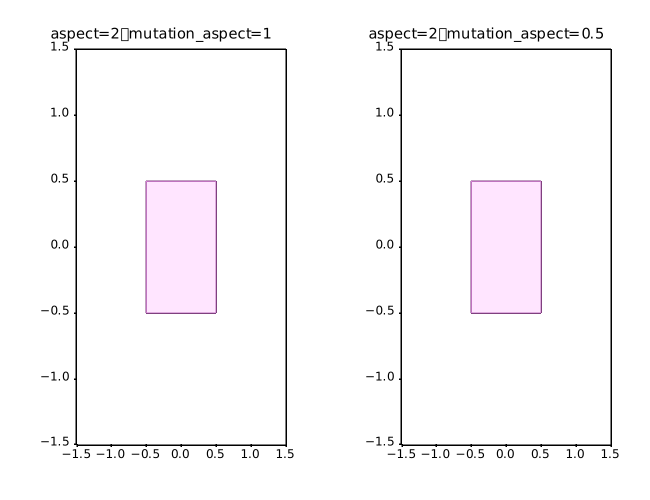
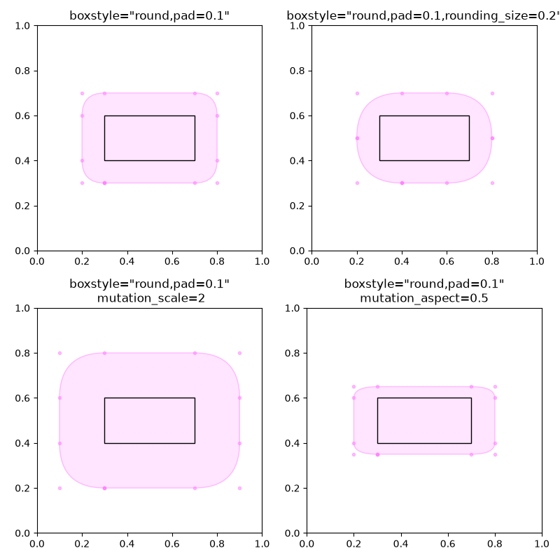
shapes_and_collections/hatch_demo
==========
Source
"""
==========
Hatch demo
==========
Hatches can be added to most polygons in Matplotlib, including `~.Axes.bar`,
`~.Axes.fill_between`, `~.Axes.contourf`, and children of `~.patches.Polygon`.
They are currently supported in the PS, PDF, SVG, macosx, and Agg backends. The WX
and Cairo backends do not currently support hatching.
See also :doc:`/gallery/images_contours_and_fields/contourf_hatching` for
an example using `~.Axes.contourf`, and
:doc:`/gallery/shapes_and_collections/hatch_style_reference` for swatches
of the existing hatches.
"""
import matplotlib.pyplot as plt
import numpy as np
from matplotlib.patches import Ellipse, Polygon
x = np.arange(1, 5)
y1 = np.arange(1, 5)
y2 = np.ones(y1.shape) * 4
fig = plt.figure()
axs = fig.subplot_mosaic([['bar1', 'patches'], ['bar2', 'patches']])
axs['bar1'].bar(x, y1, edgecolor='black', hatch="/")
axs['bar1'].bar(x, y2, bottom=y1, edgecolor='black', hatch='//')
axs['bar2'].bar(x, y1, edgecolor='black', hatch=['--', '+', 'x', '\\'])
axs['bar2'].bar(x, y2, bottom=y1, edgecolor='black',
hatch=['*', 'o', 'O', '.'])
x = np.arange(0, 40, 0.2)
axs['patches'].fill_between(x, np.sin(x) * 4 + 30, y2=0,
hatch='///', zorder=2, fc='c')
axs['patches'].add_patch(Ellipse((4, 50), 10, 10, fill=True,
hatch='*', facecolor='y'))
axs['patches'].add_patch(Polygon([(10, 20), (30, 50), (50, 10)],
hatch=r'\/...', facecolor='g'))
axs['patches'].set_xlim(0, 40)
axs['patches'].set_ylim(10, 60)
axs['patches'].set_aspect(1)
plt.show()
# %%
#
# .. admonition:: References
#
# The use of the following functions, methods, classes and modules is shown
# in this example:
#
# - `matplotlib.patches`
# - `matplotlib.patches.Ellipse`
# - `matplotlib.patches.Polygon`
# - `matplotlib.axes.Axes.add_patch`
# - `matplotlib.patches.Patch.set_hatch`
# - `matplotlib.axes.Axes.bar` / `matplotlib.pyplot.bar`
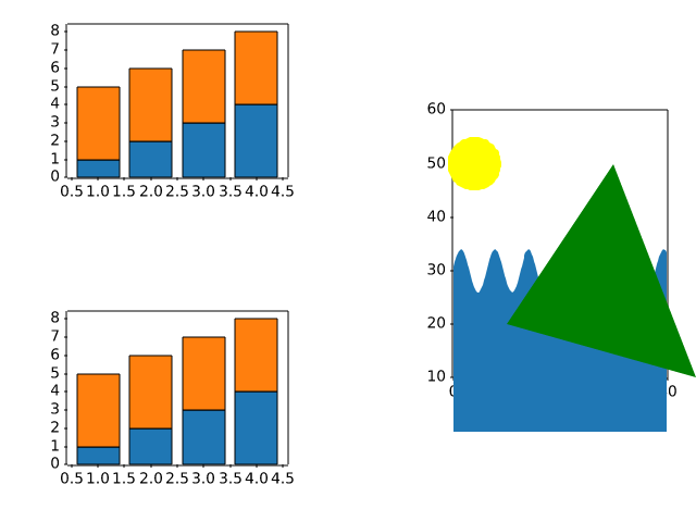
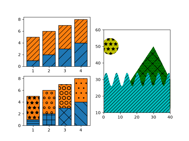
shapes_and_collections/hatch_style_reference
.. _hatch_def:
Source
"""
.. _hatch_def:
=====================
Hatch style reference
=====================
Hatches can be added to most polygons in Matplotlib, including `~.Axes.bar`,
`~.Axes.fill_between`, `~.Axes.contourf`, and children of `~.patches.Polygon`.
They are currently supported in the PS, PDF, SVG, macosx, and Agg backends. The WX
and Cairo backends do not currently support hatching.
See also :doc:`/gallery/images_contours_and_fields/contourf_hatching` for
an example using `~.Axes.contourf`, and
:doc:`/gallery/shapes_and_collections/hatch_demo` for more usage examples.
"""
import matplotlib.pyplot as plt
from matplotlib.patches import Rectangle
fig, axs = plt.subplots(2, 5, layout='constrained', figsize=(6.4, 3.2))
hatches = ['/', '\\', '|', '-', '+', 'x', 'o', 'O', '.', '*']
def hatches_plot(ax, h):
ax.add_patch(Rectangle((0, 0), 2, 2, fill=False, hatch=h))
ax.text(1, -0.5, f"' {h} '", size=15, ha="center")
ax.axis('equal')
ax.axis('off')
for ax, h in zip(axs.flat, hatches):
hatches_plot(ax, h)
# %%
# Hatching patterns can be repeated to increase the density.
#
# .. note::
# In regular (non-raw) Python strings, backslashes must be escaped:
# ``'\\\\'`` and ``r'\\'`` are both the two-character hatch ``\\``.
# Forgetting this silently halves the density — ``'\\\\\\'`` is only a
# triple hatch and thus sparser than ``'//////'``.
fig, axs = plt.subplots(2, 5, layout='constrained', figsize=(6.4, 3.2))
hatches = ['//', r'\\', '||', '--', '++', 'xx', 'oo', 'OO', '..', '**']
for ax, h in zip(axs.flat, hatches):
hatches_plot(ax, h)
# %%
# Hatching patterns can be combined to create additional patterns.
fig, axs = plt.subplots(2, 5, layout='constrained', figsize=(6.4, 3.2))
hatches = ['/o', r'\|', '|*', r'\-', '+o', 'x*', 'o-', 'O|', 'O.', '*-']
for ax, h in zip(axs.flat, hatches):
hatches_plot(ax, h)
# %%
#
# .. admonition:: References
#
# The use of the following functions, methods, classes and modules is shown
# in this example:
#
# - `matplotlib.patches`
# - `matplotlib.patches.Rectangle`
# - `matplotlib.axes.Axes.add_patch`
# - `matplotlib.axes.Axes.text`
#
# .. tags::
#
# purpose: reference
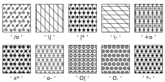
shapes_and_collections/hatchcolor_demo
===============
Source
"""
===============
Hatchcolor Demo
===============
The color of the hatch can be set using the *hatchcolor* parameter. The following
examples show how to use the *hatchcolor* parameter to set the color of the hatch
in `~.patches.Patch` and `~.collections.Collection`.
See also :doc:`/gallery/shapes_and_collections/hatch_demo` for more usage examples
of hatching.
Patch Hatchcolor
----------------
This example shows how to use the *hatchcolor* parameter to set the color of
the hatch in a rectangle and a bar plot. The *hatchcolor* parameter is available for
`~.patches.Patch`, child classes of Patch, and methods that pass through to Patch.
"""
import matplotlib.pyplot as plt
import numpy as np
import matplotlib.cm as cm
from matplotlib.patches import Rectangle
fig, (ax1, ax2) = plt.subplots(1, 2)
# Rectangle with red hatch color and black edge color
ax1.add_patch(Rectangle((0.1, 0.5), 0.8, 0.3, hatch=".", hatchcolor='red',
edgecolor='black', lw=2))
# If hatchcolor is not passed, the hatch will match the edge color
ax1.add_patch(Rectangle((0.1, 0.1), 0.8, 0.3, hatch='x', edgecolor='orange', lw=2))
x = np.arange(1, 5)
y = np.arange(1, 5)
ax2.bar(x, y, facecolor='none', edgecolor='red', hatch='//', hatchcolor='blue')
ax2.set_xlim(0, 5)
ax2.set_ylim(0, 5)
# %%
# Collection Hatchcolor
# ---------------------
#
# The following example shows how to use the *hatchcolor* parameter to set the color of
# the hatch in a scatter plot. The *hatchcolor* parameter can also be passed to
# `~.collections.Collection`, child classes of Collection, and methods that pass
# through to Collection.
fig, ax = plt.subplots()
num_points_x = 10
num_points_y = 9
x = np.linspace(0, 1, num_points_x)
y = np.linspace(0, 1, num_points_y)
X, Y = np.meshgrid(x, y)
X[1::2, :] += (x[1] - x[0]) / 2 # stagger every alternate row
# As ax.scatter (PathCollection) is drawn row by row, setting hatchcolors to the
# first row is enough, as the colors will be cycled through for the next rows.
colors = [cm.rainbow(val) for val in x]
ax.scatter(
X.ravel(),
Y.ravel(),
s=1700,
facecolor="none",
edgecolor="gray",
linewidth=2,
marker="h", # Use hexagon as marker
hatch="xxx",
hatchcolor=colors,
)
ax.set_xlim(0, 1)
ax.set_ylim(0, 1)
plt.show()
# %%
#
# .. admonition:: References
#
# The use of the following functions, methods, classes and modules is shown
# in this example:
#
# - `matplotlib.patches`
# - `matplotlib.patches.Polygon`
# - `matplotlib.axes.Axes.add_patch`
# - `matplotlib.axes.Axes.bar` / `matplotlib.pyplot.bar`
# - `matplotlib.collections`
# - `matplotlib.axes.Axes.scatter` / `matplotlib.pyplot.scatter`
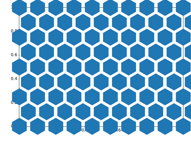
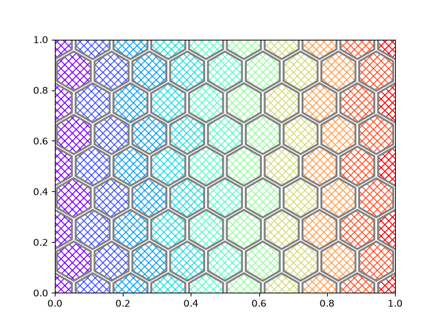
shapes_and_collections/line_collection
==========================================
Source
"""
==========================================
Plot multiple lines using a LineCollection
==========================================
Matplotlib can efficiently draw multiple lines at once using a `~.LineCollection`.
"""
import matplotlib.pyplot as plt
import numpy as np
from matplotlib.collections import LineCollection
colors = ["indigo", "blue", "green", "yellow", "orange", "red"]
# create a list of half-circles with varying radii
theta = np.linspace(0, np.pi, 36)
radii = np.linspace(4, 5, num=len(colors))
arcs = [np.column_stack([r * np.cos(theta), r * np.sin(theta)]) for r in radii]
fig, ax = plt.subplots(figsize=(6.4, 3.2))
# set axes limits manually because Collections do not take part in autoscaling
ax.set_xlim(-6, 6)
ax.set_ylim(0, 6)
ax.set_aspect("equal") # to make the arcs look circular
# create a LineCollection with the half-circles
# its properties can be set per line by passing a sequence (here used for *colors*)
# or they can be set for all lines by passing a scalar (here used for *linewidths*)
line_collection = LineCollection(arcs, colors=colors, linewidths=4)
ax.add_collection(line_collection)
plt.show()
# %%
# Instead of passing a list of colors (``colors=colors``), we can alternatively use
# colormapping. The lines are then color-coded based on an additional array of values
# passed to the *array* parameter. In the below example, we color the lines based on
# their radius by passing ``array=radii``.
num_arcs = 15
theta = np.linspace(0, np.pi, 36)
radii = np.linspace(4, 5.5, num=num_arcs)
arcs = [np.column_stack([r * np.cos(theta), r * np.sin(theta)]) for r in radii]
fig, ax = plt.subplots(figsize=(6.4, 3))
# set axes limits manually because Collections do not take part in autoscaling
ax.set_xlim(-6, 6)
ax.set_ylim(0, 6)
ax.set_aspect("equal") # to make the arcs look circular
# create a LineCollection with the half-circles and color mapping
line_collection = LineCollection(arcs, array=radii, cmap="rainbow")
ax.add_collection(line_collection)
fig.colorbar(line_collection, label="Radius")
ax.set_title("Line Collection with mapped colors")
plt.show()
# %%
#
# .. admonition:: References
#
# The use of the following functions, methods, classes and modules is shown
# in this example:
#
# - `matplotlib.collections.LineCollection`
# - `matplotlib.collections.Collection.set_array`
# - `matplotlib.axes.Axes.add_collection`
# - `matplotlib.figure.Figure.colorbar` / `matplotlib.pyplot.colorbar`
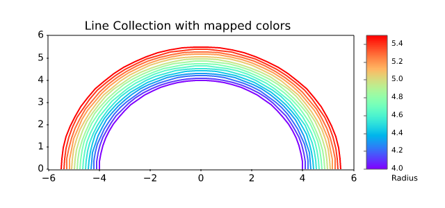
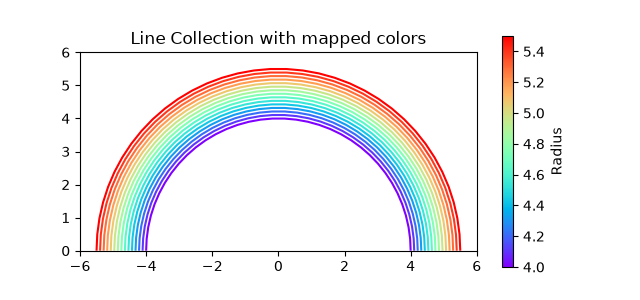
shapes_and_collections/patch_collection
============================
Source
"""
============================
Circles, Wedges and Polygons
============================
This example demonstrates how to use `.collections.PatchCollection`.
See also :doc:`/gallery/shapes_and_collections/artist_reference`, which instead
adds each artist separately to its own Axes.
"""
import matplotlib.pyplot as plt
import numpy as np
from matplotlib.collections import PatchCollection
from matplotlib.patches import Circle, Polygon, Wedge
# Fixing random state for reproducibility
np.random.seed(19680801)
fig, ax = plt.subplots()
resolution = 50 # the number of vertices
N = 3
x = np.random.rand(N)
y = np.random.rand(N)
radii = 0.1*np.random.rand(N)
patches = []
for x1, y1, r in zip(x, y, radii):
circle = Circle((x1, y1), r)
patches.append(circle)
x = np.random.rand(N)
y = np.random.rand(N)
radii = 0.1*np.random.rand(N)
theta1 = 360.0*np.random.rand(N)
theta2 = 360.0*np.random.rand(N)
for x1, y1, r, t1, t2 in zip(x, y, radii, theta1, theta2):
wedge = Wedge((x1, y1), r, t1, t2)
patches.append(wedge)
# Some limiting conditions on Wedge
patches += [
Wedge((.3, .7), .1, 0, 360), # Full circle
Wedge((.7, .8), .2, 0, 360, width=0.05), # Full ring
Wedge((.8, .3), .2, 0, 45), # Full sector
Wedge((.8, .3), .2, 45, 90, width=0.10), # Ring sector
]
for i in range(N):
polygon = Polygon(np.random.rand(N, 2), closed=True)
patches.append(polygon)
colors = 100 * np.random.rand(len(patches))
p = PatchCollection(patches, alpha=0.4)
p.set_array(colors)
ax.add_collection(p)
fig.colorbar(p, ax=ax)
plt.show()
# %%
#
# .. admonition:: References
#
# The use of the following functions, methods, classes and modules is shown
# in this example:
#
# - `matplotlib.patches`
# - `matplotlib.patches.Circle`
# - `matplotlib.patches.Wedge`
# - `matplotlib.patches.Polygon`
# - `matplotlib.collections.PatchCollection`
# - `matplotlib.collections.Collection.set_array`
# - `matplotlib.axes.Axes.add_collection`
# - `matplotlib.figure.Figure.colorbar`
shapes_and_collections/path_patch
================
Source
r"""
================
PathPatch object
================
This example shows how to create `~.path.Path` and `~.patches.PathPatch`
objects through Matplotlib's API.
"""
import matplotlib.pyplot as plt
import matplotlib.patches as mpatches
import matplotlib.path as mpath
fig, ax = plt.subplots()
Path = mpath.Path
path_data = [
(Path.MOVETO, (1.58, -2.57)),
(Path.CURVE4, (0.35, -1.1)),
(Path.CURVE4, (-1.75, 2.0)),
(Path.CURVE4, (0.375, 2.0)),
(Path.LINETO, (0.85, 1.15)),
(Path.CURVE4, (2.2, 3.2)),
(Path.CURVE4, (3, 0.05)),
(Path.CURVE4, (2.0, -0.5)),
(Path.CLOSEPOLY, (1.58, -2.57)),
]
codes, verts = zip(*path_data)
path = mpath.Path(verts, codes)
patch = mpatches.PathPatch(path, facecolor='r', alpha=0.5)
ax.add_patch(patch)
# plot control points and connecting lines
x, y = zip(*path.vertices)
line, = ax.plot(x, y, 'go-')
ax.grid()
ax.axis('equal')
plt.show()
# %%
#
# .. admonition:: References
#
# The use of the following functions, methods, classes and modules is shown
# in this example:
#
# - `matplotlib.path`
# - `matplotlib.path.Path`
# - `matplotlib.patches`
# - `matplotlib.patches.PathPatch`
# - `matplotlib.axes.Axes.add_patch`
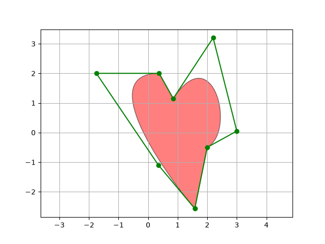
shapes_and_collections/quad_bezier
============
Source
"""
============
Bezier curve
============
This example showcases the `~.patches.PathPatch` object to create a Bezier
polycurve path patch.
"""
import matplotlib.pyplot as plt
import matplotlib.patches as mpatches
import matplotlib.path as mpath
Path = mpath.Path
fig, ax = plt.subplots()
pp1 = mpatches.PathPatch(
Path([(0, 0), (1, 0), (1, 1), (0, 0)],
[Path.MOVETO, Path.CURVE3, Path.CURVE3, Path.CLOSEPOLY]),
fc="none", transform=ax.transData)
ax.add_patch(pp1)
ax.plot([0.75], [0.25], "ro")
ax.set_title('The red point should be on the path')
plt.show()
# %%
#
# .. admonition:: References
#
# The use of the following functions, methods, classes and modules is shown
# in this example:
#
# - `matplotlib.path`
# - `matplotlib.path.Path`
# - `matplotlib.patches`
# - `matplotlib.patches.PathPatch`
# - `matplotlib.axes.Axes.add_patch`
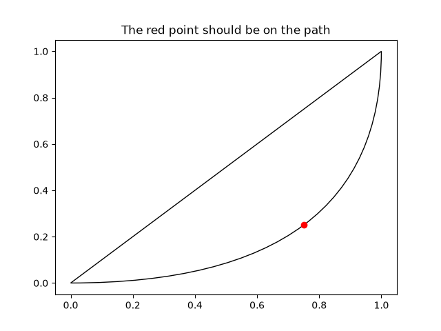
shapes_and_collections/scatter
============
Source
""" ============ Scatter plot ============ This example showcases a simple scatter plot. """ import matplotlib.pyplot as plt import numpy as np # Fixing random state for reproducibility np.random.seed(19680801) N = 50 x = np.random.rand(N) y = np.random.rand(N) colors = np.random.rand(N) area = (30 * np.random.rand(N))**2 # 0 to 15 point radii plt.scatter(x, y, s=area, c=colors, alpha=0.5) plt.show() # %% # # .. admonition:: References # # The use of the following functions, methods, classes and modules is shown # in this example: # # - `matplotlib.axes.Axes.scatter` / `matplotlib.pyplot.scatter`
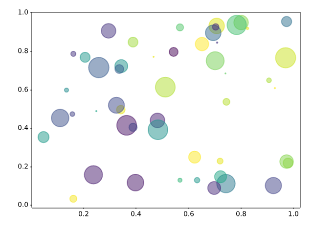
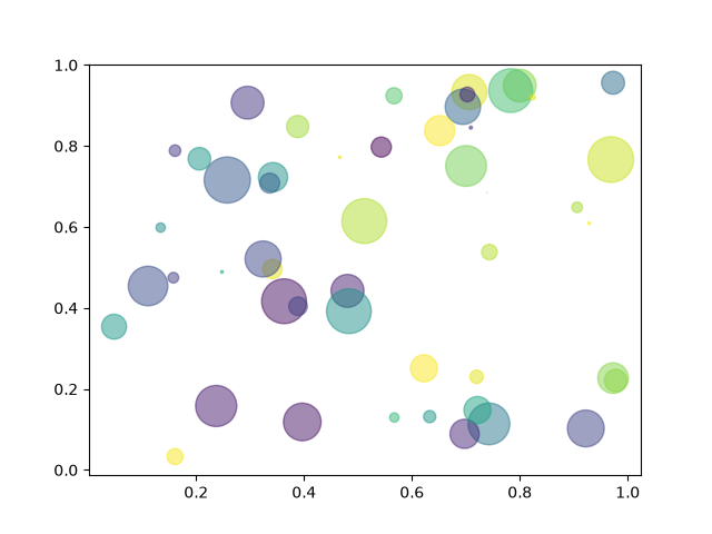
showcase/anatomy
===================
Source
"""
===================
Anatomy of a figure
===================
This figure shows the name of several matplotlib elements composing a figure
"""
import matplotlib.pyplot as plt
import numpy as np
from matplotlib.patches import Circle
from matplotlib.patheffects import withStroke
from matplotlib.ticker import AutoMinorLocator, MultipleLocator
royal_blue = [0, 20/256, 82/256]
# make the figure
np.random.seed(19680801)
X = np.linspace(0.5, 3.5, 100)
Y1 = 3+np.cos(X)
Y2 = 1+np.cos(1+X/0.75)/2
Y3 = np.random.uniform(Y1, Y2, len(X))
fig = plt.figure(figsize=(7.5, 7.5))
ax = fig.add_axes((0.2, 0.17, 0.68, 0.7), aspect=1)
ax.xaxis.set_major_locator(MultipleLocator(1.000))
ax.xaxis.set_minor_locator(AutoMinorLocator(4))
ax.yaxis.set_major_locator(MultipleLocator(1.000))
ax.yaxis.set_minor_locator(AutoMinorLocator(4))
ax.xaxis.set_minor_formatter("{x:.2f}")
ax.set_xlim(0, 4)
ax.set_ylim(0, 4)
ax.tick_params(which='major', width=1.0, length=10, labelsize=14)
ax.tick_params(which='minor', width=1.0, length=5, labelsize=10,
labelcolor='0.25')
ax.grid(linestyle="--", linewidth=0.5, color='.25', zorder=-10)
ax.plot(X, Y1, c='C0', lw=2.5, label="Blue signal", zorder=10)
ax.plot(X, Y2, c='C1', lw=2.5, label="Orange signal")
ax.plot(X[::3], Y3[::3], linewidth=0, markersize=9,
marker='s', markerfacecolor='none', markeredgecolor='C4',
markeredgewidth=2.5)
ax.set_title("Anatomy of a figure", fontsize=20, verticalalignment='bottom')
ax.set_xlabel("x Axis label", fontsize=14)
ax.set_ylabel("y Axis label", fontsize=14)
ax.legend(loc="upper right", fontsize=14)
# Annotate the figure
def annotate(x, y, text, code):
# Circle marker
c = Circle((x, y), radius=0.15, clip_on=False, zorder=10, linewidth=2.5,
edgecolor=royal_blue + [0.6], facecolor='none',
path_effects=[withStroke(linewidth=7, foreground='white')])
ax.add_artist(c)
# use path_effects as a background for the texts
# draw the path_effects and the colored text separately so that the
# path_effects cannot clip other texts
for path_effects in [[withStroke(linewidth=7, foreground='white')], []]:
color = 'white' if path_effects else royal_blue
ax.text(x, y-0.2, text, zorder=100,
ha='center', va='top', weight='bold', color=color,
style='italic', fontfamily='monospace',
path_effects=path_effects)
color = 'white' if path_effects else 'black'
ax.text(x, y-0.33, code, zorder=100,
ha='center', va='top', weight='normal', color=color,
fontfamily='monospace', fontsize='medium',
path_effects=path_effects)
annotate(3.5, -0.13, "Minor tick label", "ax.xaxis.set_minor_formatter")
annotate(-0.03, 1.0, "Major tick", "ax.yaxis.set_major_locator")
annotate(0.00, 3.75, "Minor tick", "ax.yaxis.set_minor_locator")
annotate(-0.15, 3.00, "Major tick label", "ax.yaxis.set_major_formatter")
annotate(1.68, -0.39, "xlabel", "ax.set_xlabel")
annotate(-0.38, 1.67, "ylabel", "ax.set_ylabel")
annotate(1.52, 4.15, "Title", "ax.set_title")
annotate(1.75, 2.80, "Line", "ax.plot")
annotate(2.25, 1.54, "Markers", "ax.scatter")
annotate(3.00, 3.00, "Grid", "ax.grid")
annotate(3.60, 3.58, "Legend", "ax.legend")
annotate(2.5, 0.55, "Axes", "fig.subplots")
annotate(4, 4.5, "Figure", "plt.figure")
annotate(0.65, 0.01, "x Axis", "ax.xaxis")
annotate(0, 0.36, "y Axis", "ax.yaxis")
annotate(4.0, 0.7, "Spine", "ax.spines")
# frame around figure
fig.patch.set(linewidth=4, edgecolor='0.5')
plt.show()
# %%
#
# .. admonition:: References
#
# The use of the following functions, methods, classes and modules is shown
# in this example:
#
# - `matplotlib.pyplot.figure`
# - `matplotlib.axes.Axes.text`
# - `matplotlib.axis.Axis.set_minor_formatter`
# - `matplotlib.axis.Axis.set_major_locator`
# - `matplotlib.axis.Axis.set_minor_locator`
# - `matplotlib.patches.Circle`
# - `matplotlib.patheffects.withStroke`
# - `matplotlib.ticker.FuncFormatter`
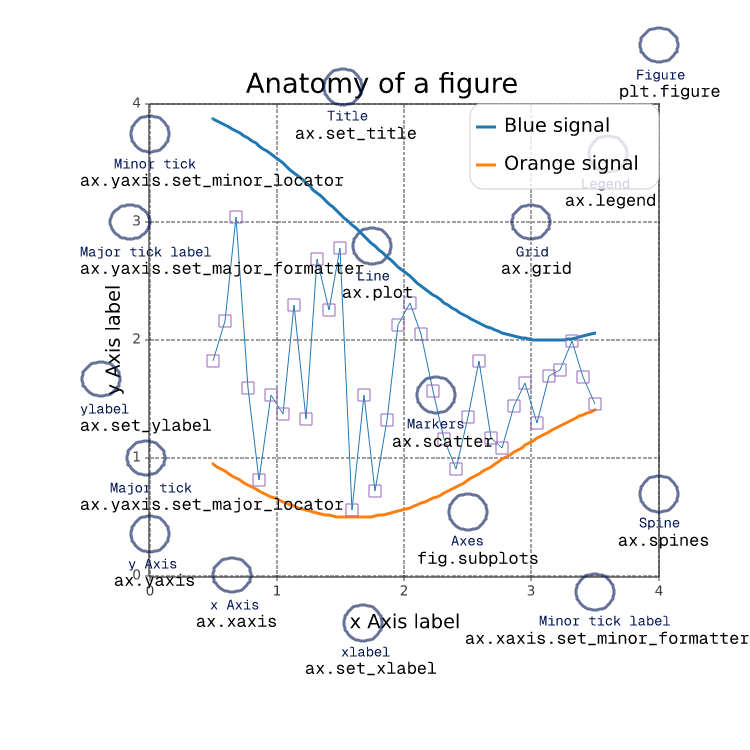
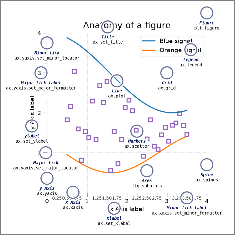
showcase/firefox
=======
Source
"""
=======
Firefox
=======
This example shows how to create the Firefox logo with path and patches.
"""
import re
import matplotlib.pyplot as plt
import numpy as np
import matplotlib.patches as patches
from matplotlib.path import Path
# From: https://dmitrybaranovskiy.github.io/raphael/icons/#firefox
firefox = "M28.4,22.469c0.479-0.964,0.851-1.991,1.095-3.066c0.953-3.661,0.666-6.854,0.666-6.854l-0.327,2.104c0,0-0.469-3.896-1.044-5.353c-0.881-2.231-1.273-2.214-1.274-2.21c0.542,1.379,0.494,2.169,0.483,2.288c-0.01-0.016-0.019-0.032-0.027-0.047c-0.131-0.324-0.797-1.819-2.225-2.878c-2.502-2.481-5.943-4.014-9.745-4.015c-4.056,0-7.705,1.745-10.238,4.525C5.444,6.5,5.183,5.938,5.159,5.317c0,0-0.002,0.002-0.006,0.005c0-0.011-0.003-0.021-0.003-0.031c0,0-1.61,1.247-1.436,4.612c-0.299,0.574-0.56,1.172-0.777,1.791c-0.375,0.817-0.75,2.004-1.059,3.746c0,0,0.133-0.422,0.399-0.988c-0.064,0.482-0.103,0.971-0.116,1.467c-0.09,0.845-0.118,1.865-0.039,3.088c0,0,0.032-0.406,0.136-1.021c0.834,6.854,6.667,12.165,13.743,12.165l0,0c1.86,0,3.636-0.37,5.256-1.036C24.938,27.771,27.116,25.196,28.4,22.469zM16.002,3.356c2.446,0,4.73,0.68,6.68,1.86c-2.274-0.528-3.433-0.261-3.423-0.248c0.013,0.015,3.384,0.589,3.981,1.411c0,0-1.431,0-2.856,0.41c-0.065,0.019,5.242,0.663,6.327,5.966c0,0-0.582-1.213-1.301-1.42c0.473,1.439,0.351,4.17-0.1,5.528c-0.058,0.174-0.118-0.755-1.004-1.155c0.284,2.037-0.018,5.268-1.432,6.158c-0.109,0.07,0.887-3.189,0.201-1.93c-4.093,6.276-8.959,2.539-10.934,1.208c1.585,0.388,3.267,0.108,4.242-0.559c0.982-0.672,1.564-1.162,2.087-1.047c0.522,0.117,0.87-0.407,0.464-0.872c-0.405-0.466-1.392-1.105-2.725-0.757c-0.94,0.247-2.107,1.287-3.886,0.233c-1.518-0.899-1.507-1.63-1.507-2.095c0-0.366,0.257-0.88,0.734-1.028c0.58,0.062,1.044,0.214,1.537,0.466c0.005-0.135,0.006-0.315-0.001-0.519c0.039-0.077,0.015-0.311-0.047-0.596c-0.036-0.287-0.097-0.582-0.19-0.851c0.01-0.002,0.017-0.007,0.021-0.021c0.076-0.344,2.147-1.544,2.299-1.659c0.153-0.114,0.55-0.378,0.506-1.183c-0.015-0.265-0.058-0.294-2.232-0.286c-0.917,0.003-1.425-0.894-1.589-1.245c0.222-1.231,0.863-2.11,1.919-2.704c0.02-0.011,0.015-0.021-0.008-0.027c0.219-0.127-2.524-0.006-3.76,1.604C9.674,8.045,9.219,7.95,8.71,7.95c-0.638,0-1.139,0.07-1.603,0.187c-0.05,0.013-0.122,0.011-0.208-0.001C6.769,8.04,6.575,7.88,6.365,7.672c0.161-0.18,0.324-0.356,0.495-0.526C9.201,4.804,12.43,3.357,16.002,3.356z" # noqa
def svg_parse(path):
commands = {'M': (Path.MOVETO,),
'L': (Path.LINETO,),
'Q': (Path.CURVE3,)*2,
'C': (Path.CURVE4,)*3,
'Z': (Path.CLOSEPOLY,)}
vertices = []
codes = []
cmd_values = re.split("([A-Za-z])", path)[1:] # Split over commands.
for cmd, values in zip(cmd_values[::2], cmd_values[1::2]):
# Numbers are separated either by commas, or by +/- signs (but not at
# the beginning of the string).
points = ([*map(float, re.split(",|(?<!^)(?=[+-])", values))] if values
else [(0., 0.)]) # Only for "z/Z" (CLOSEPOLY).
points = np.reshape(points, (-1, 2))
if cmd.islower():
points += vertices[-1][-1]
codes.extend(commands[cmd.upper()])
vertices.append(points)
return np.array(codes), np.concatenate(vertices)
# SVG to Matplotlib
codes, verts = svg_parse(firefox)
path = Path(verts, codes)
xmin, ymin = verts.min(axis=0) - 1
xmax, ymax = verts.max(axis=0) + 1
fig = plt.figure(figsize=(5, 5), facecolor="0.75") # gray background
ax = fig.add_axes((0, 0, 1, 1), frameon=False, aspect=1,
xlim=(xmin, xmax), # centering
ylim=(ymax, ymin), # centering, upside down
xticks=[], yticks=[]) # no ticks
# White outline (width = 6)
ax.add_patch(patches.PathPatch(path, facecolor='none', edgecolor='w', lw=6))
# Actual shape with black outline
ax.add_patch(patches.PathPatch(path, facecolor='orange', edgecolor='k', lw=2))
plt.show() # Display
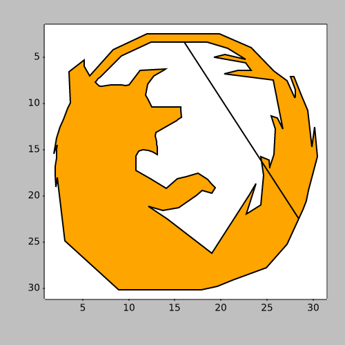

showcase/integral
==================================
Source
"""
==================================
Integral as the area under a curve
==================================
Although this is a simple example, it demonstrates some important tweaks:
* A simple line plot with custom color and line width.
* A shaded region created using a Polygon patch.
* A text label with mathtext rendering.
* figtext calls to label the x- and y-axes.
* Use of axis spines to hide the top and right spines.
* Custom tick placement and labels.
"""
import matplotlib.pyplot as plt
import numpy as np
from matplotlib.patches import Polygon
def func(x):
return (x - 3) * (x - 5) * (x - 7) + 85
a, b = 2, 9 # integral limits
x = np.linspace(0, 10)
y = func(x)
fig, ax = plt.subplots()
ax.plot(x, y, 'r', linewidth=2)
ax.set_ylim(bottom=0)
# Make the shaded region
ix = np.linspace(a, b)
iy = func(ix)
verts = [(a, 0), *zip(ix, iy), (b, 0)]
poly = Polygon(verts, facecolor='0.9', edgecolor='0.5')
ax.add_patch(poly)
ax.text(0.5 * (a + b), 30, r"$\int_a^b f(x)\mathrm{d}x$",
horizontalalignment='center', fontsize=20)
fig.text(0.9, 0.05, '$x$')
fig.text(0.1, 0.9, '$y$')
ax.spines[['top', 'right']].set_visible(False)
ax.set_xticks([a, b], labels=['$a$', '$b$'])
ax.set_yticks([])
plt.show()
showcase/mandelbrot
===================================
Source
"""
===================================
Shaded & power normalized rendering
===================================
The Mandelbrot set rendering can be improved by using a normalized recount
associated with a power normalized colormap (gamma=0.3). Rendering can be
further enhanced thanks to shading.
The ``maxiter`` gives the precision of the computation. ``maxiter=200`` should
take a few seconds on most modern laptops.
"""
import numpy as np
def mandelbrot_set(xmin, xmax, ymin, ymax, xn, yn, maxiter, horizon=2.0):
X = np.linspace(xmin, xmax, xn).astype(np.float32)
Y = np.linspace(ymin, ymax, yn).astype(np.float32)
C = X + Y[:, None] * 1j
N = np.zeros_like(C, dtype=int)
Z = np.zeros_like(C)
for n in range(maxiter):
I = abs(Z) < horizon
N[I] = n
Z[I] = Z[I]**2 + C[I]
N[N == maxiter-1] = 0
return Z, N
if __name__ == '__main__':
import time
import matplotlib.pyplot as plt
import matplotlib
from matplotlib import colors
xmin, xmax, xn = -2.25, +0.75, 3000 // 2
ymin, ymax, yn = -1.25, +1.25, 2500 // 2
maxiter = 200
horizon = 2.0 ** 40
log_horizon = np.log2(np.log(horizon))
Z, N = mandelbrot_set(xmin, xmax, ymin, ymax, xn, yn, maxiter, horizon)
# Normalized recount as explained in:
# https://linas.org/art-gallery/escape/smooth.html
# https://web.archive.org/web/20160331171238/https://www.ibm.com/developerworks/community/blogs/jfp/entry/My_Christmas_Gift?lang=en
# This line will generate warnings for null values, but it is faster to
# process them afterwards using the nan_to_num
with np.errstate(invalid='ignore'):
M = np.nan_to_num(N + 1 - np.log2(np.log(abs(Z))) + log_horizon)
dpi = 72
width = 10
height = 10*yn/xn
fig = plt.figure(figsize=(width, height), dpi=dpi)
ax = fig.add_axes((0, 0, 1, 1), frameon=False, aspect=1)
# Shaded rendering
light = colors.LightSource(azdeg=315, altdeg=10)
M = light.shade(M, cmap=plt.colormaps["hot"], vert_exag=1.5,
norm=colors.PowerNorm(0.3), blend_mode='hsv')
ax.imshow(M, extent=[xmin, xmax, ymin, ymax], interpolation="bicubic")
ax.set_xticks([])
ax.set_yticks([])
# Some advertisement for matplotlib
year = time.strftime("%Y")
text = ("The Mandelbrot fractal set\n"
"Rendered with matplotlib %s, %s - https://matplotlib.org"
% (matplotlib.__version__, year))
ax.text(xmin+.025, ymin+.025, text, color="white", fontsize=12, alpha=0.5)
plt.show()
showcase/pan_zoom_overlap
===================================
Source
"""
===================================
Pan/zoom events of overlapping axes
===================================
Example to illustrate how pan/zoom events of overlapping axes are treated.
The default is the following:
- Axes with a visible patch capture pan/zoom events
- Axes with an invisible patch forward pan/zoom events to axes below
- Shared axes always trigger with their parent axes
(irrespective of the patch visibility)
Note: The visibility of the patch hereby refers to the value of
``ax.patch.get_visible()``. The color and transparency of a
patch have no effect on the treatment of pan/zoom events!
``ax.set_forward_navigation_events(val)`` can be used to override the
default behaviour:
- ``True``: Forward navigation events to axes below.
- ``False``: Execute navigation events only on this axes.
- ``"auto"``: Use the default behaviour.
To disable pan/zoom events completely, use ``ax.set_navigate(False)``
"""
import matplotlib.pyplot as plt
fig = plt.figure(figsize=(11, 6))
fig.suptitle("Showcase for pan/zoom events on overlapping axes.")
ax = fig.add_axes((.05, .05, .9, .9))
ax.patch.set_color(".75")
ax_twin = ax.twinx()
ax1 = fig.add_subplot(221)
ax1_twin = ax1.twinx()
ax1.text(.5, .5,
"Visible patch\n\n"
"Pan/zoom events are NOT\n"
"forwarded to axes below",
ha="center", va="center", transform=ax1.transAxes)
ax11 = fig.add_subplot(223, sharex=ax1, sharey=ax1)
ax11.set_forward_navigation_events(True)
ax11.text(.5, .5,
"Visible patch\n\n"
"Override capture behavior:\n\n"
"ax.set_forward_navigation_events(True)",
ha="center", va="center", transform=ax11.transAxes)
ax2 = fig.add_subplot(222)
ax2_twin = ax2.twinx()
ax2.patch.set_visible(False)
ax2.text(.5, .5,
"Invisible patch\n\n"
"Pan/zoom events are\n"
"forwarded to axes below",
ha="center", va="center", transform=ax2.transAxes)
ax22 = fig.add_subplot(224, sharex=ax2, sharey=ax2)
ax22.patch.set_visible(False)
ax22.set_forward_navigation_events(False)
ax22.text(.5, .5,
"Invisible patch\n\n"
"Override capture behavior:\n\n"
"ax.set_forward_navigation_events(False)",
ha="center", va="center", transform=ax22.transAxes)
showcase/stock_prices
==========================
Source
"""
==========================
Stock prices over 32 years
==========================
.. redirect-from:: /gallery/showcase/bachelors_degrees_by_gender
A graph of multiple time series that demonstrates custom styling of plot frame,
tick lines, tick labels, and line graph properties. It also uses custom
placement of text labels along the right edge as an alternative to a
conventional legend.
Note: The third-party mpl style dufte_ produces similar-looking plots with less
code.
.. _dufte: https://github.com/nschloe/dufte
"""
import matplotlib.pyplot as plt
import numpy as np
from matplotlib.cbook import get_sample_data
import matplotlib.transforms as mtransforms
with get_sample_data('Stocks.csv') as file:
stock_data = np.genfromtxt(
file, delimiter=',', names=True, dtype=None,
converters={0: lambda x: np.datetime64(x, 'D')}, skip_header=1)
fig, ax = plt.subplots(1, 1, figsize=(6, 8), layout='constrained')
# These are the colors that will be used in the plot
ax.set_prop_cycle(color=[
'#1f77b4', '#aec7e8', '#ff7f0e', '#ffbb78', '#2ca02c', '#98df8a',
'#d62728', '#ff9896', '#9467bd', '#c5b0d5', '#8c564b', '#c49c94',
'#e377c2', '#f7b6d2', '#7f7f7f', '#c7c7c7', '#bcbd22', '#dbdb8d',
'#17becf', '#9edae5'])
stocks_name = ['IBM', 'Apple', 'Microsoft', 'Xerox', 'Amazon', 'Dell',
'Alphabet', 'Adobe', 'S&P 500', 'NASDAQ']
stocks_ticker = ['IBM', 'AAPL', 'MSFT', 'XRX', 'AMZN', 'DELL', 'GOOGL',
'ADBE', 'GSPC', 'IXIC']
# Manually adjust the label positions vertically (units are points = 1/72 inch)
y_offsets = dict.fromkeys(stocks_ticker, 0)
y_offsets['IBM'] = 5
y_offsets['AAPL'] = -5
y_offsets['AMZN'] = -6
for nn, column in enumerate(stocks_ticker):
# Plot each line separately with its own color.
# don't include any data with NaN.
good = np.nonzero(np.isfinite(stock_data[column]))
line, = ax.plot(stock_data['Date'][good], stock_data[column][good], lw=2.5)
# Add a text label to the right end of every line. Most of the code below
# is adding specific offsets y position because some labels overlapped.
y_pos = stock_data[column][-1]
# Use an offset transform, in points, for any text that needs to be nudged
# up or down.
offset = y_offsets[column] / 72
trans = mtransforms.ScaledTranslation(0, offset, fig.dpi_scale_trans)
trans = ax.transData + trans
# Again, make sure that all labels are large enough to be easily read
# by the viewer.
ax.text(np.datetime64('2022-10-01'), y_pos, stocks_name[nn],
color=line.get_color(), transform=trans)
ax.set_xlim(np.datetime64('1989-06-01'), np.datetime64('2023-01-01'))
fig.suptitle("Technology company stocks prices dollars (1990-2022)",
ha="center")
# Remove the plot frame lines. They are unnecessary here.
ax.spines[:].set_visible(False)
# Ensure that the axis ticks only show up on the bottom and left of the plot.
# Ticks on the right and top of the plot are generally unnecessary.
ax.xaxis.tick_bottom()
ax.yaxis.tick_left()
ax.set_yscale('log')
# Provide tick lines across the plot to help your viewers trace along
# the axis ticks. Make sure that the lines are light and small so they
# don't obscure the primary data lines.
ax.grid(True, 'major', 'both', ls='--', lw=.5, c='k', alpha=.3)
# Remove the tick marks; they are unnecessary with the tick lines we just
# plotted. Make sure your axis ticks are large enough to be easily read.
# You don't want your viewers squinting to read your plot.
ax.tick_params(axis='both', which='both', labelsize='large',
bottom=False, top=False, labelbottom=True,
left=False, right=False, labelleft=True)
# Finally, save the figure as a PNG.
# You can also save it as a PDF, JPEG, etc.
# Just change the file extension in this call.
# fig.savefig('stock-prices.png', bbox_inches='tight')
plt.show()
# %%
#
# .. admonition:: References
#
# The use of the following functions, methods, classes and modules is shown
# in this example:
#
# - `matplotlib.pyplot.subplots`
# - `matplotlib.axes.Axes.text`
# - `matplotlib.axis.XAxis.tick_bottom`
# - `matplotlib.axis.YAxis.tick_left`
# - `matplotlib.artist.Artist.set_visible`
showcase/xkcd
====
Source
"""
====
XKCD
====
Shows how to create an xkcd-like plot.
"""
import matplotlib.pyplot as plt
import numpy as np
# %%
with plt.xkcd():
# Based on "Stove Ownership" from XKCD by Randall Munroe
# https://xkcd.com/418/
fig = plt.figure()
ax = fig.add_axes((0.1, 0.2, 0.8, 0.7))
ax.spines[['top', 'right']].set_visible(False)
ax.set_xticks([])
ax.set_yticks([])
ax.set_ylim(-30, 10)
data = np.ones(100)
data[70:] -= np.arange(30)
ax.annotate(
'THE DAY I REALIZED\nI COULD COOK BACON\nWHENEVER I WANTED',
xy=(70, 1), arrowprops=dict(arrowstyle='->'), xytext=(15, -10))
ax.plot(data)
ax.set_xlabel('time')
ax.set_ylabel('my overall health')
fig.text(
0.5, 0.05,
'"Stove Ownership" from xkcd by Randall Munroe',
ha='center')
# %%
with plt.xkcd():
# Based on "The Data So Far" from XKCD by Randall Munroe
# https://xkcd.com/373/
fig = plt.figure()
ax = fig.add_axes((0.1, 0.2, 0.8, 0.7))
ax.bar([0, 1], [0, 100], 0.25)
ax.spines[['top', 'right']].set_visible(False)
ax.xaxis.set_ticks_position('bottom')
ax.set_xticks([0, 1])
ax.set_xticklabels(['CONFIRMED BY\nEXPERIMENT', 'REFUTED BY\nEXPERIMENT'])
ax.set_xlim(-0.5, 1.5)
ax.set_yticks([])
ax.set_ylim(0, 110)
ax.set_title("CLAIMS OF SUPERNATURAL POWERS")
fig.text(
0.5, 0.05,
'"The Data So Far" from xkcd by Randall Munroe',
ha='center')
plt.show()
#
# %%
# .. tags::
#
# plot-type: line
# plot-type: bar
# purpose: fun
specialty_plots/advanced_hillshading
===========
Source
"""
===========
Hillshading
===========
Demonstrates a few common tricks with shaded plots.
"""
import matplotlib.pyplot as plt
import numpy as np
from matplotlib.colors import LightSource, Normalize
def display_colorbar():
"""Display a correct numeric colorbar for a shaded plot."""
y, x = np.mgrid[-4:2:200j, -4:2:200j]
z = 10 * np.cos(x**2 + y**2)
cmap = plt.colormaps["copper"]
ls = LightSource(315, 45)
rgb = ls.shade(z, cmap)
fig, ax = plt.subplots()
ax.imshow(rgb, interpolation='bilinear')
# Use a proxy artist for the colorbar...
im = ax.imshow(z, cmap=cmap)
im.remove()
fig.colorbar(im, ax=ax)
ax.set_title('Using a colorbar with a shaded plot', size='x-large')
def avoid_outliers():
"""Use a custom norm to control the displayed z-range of a shaded plot."""
y, x = np.mgrid[-4:2:200j, -4:2:200j]
z = 10 * np.cos(x**2 + y**2)
# Add some outliers...
z[100, 105] = 2000
z[120, 110] = -9000
ls = LightSource(315, 45)
fig, (ax1, ax2) = plt.subplots(ncols=2, figsize=(8, 4.5))
rgb = ls.shade(z, plt.colormaps["copper"])
ax1.imshow(rgb, interpolation='bilinear')
ax1.set_title('Full range of data')
rgb = ls.shade(z, plt.colormaps["copper"], vmin=-10, vmax=10)
ax2.imshow(rgb, interpolation='bilinear')
ax2.set_title('Manually set range')
fig.suptitle('Avoiding Outliers in Shaded Plots', size='x-large')
def shade_other_data():
"""Demonstrates displaying different variables through shade and color."""
y, x = np.mgrid[-4:2:200j, -4:2:200j]
z1 = np.sin(x**2) # Data to hillshade
z2 = np.cos(x**2 + y**2) # Data to color
norm = Normalize(z2.min(), z2.max())
cmap = plt.colormaps["RdBu"]
ls = LightSource(315, 45)
rgb = ls.shade_rgb(cmap(norm(z2)), z1)
fig, ax = plt.subplots()
ax.imshow(rgb, interpolation='bilinear')
ax.set_title('Shade by one variable, color by another', size='x-large')
display_colorbar()
avoid_outliers()
shade_other_data()
plt.show()
specialty_plots/anscombe
==================
Source
"""
==================
Anscombe's quartet
==================
`Anscombe's quartet`_ is a group of datasets (x, y) that have the same mean,
standard deviation, and regression line, but which are qualitatively different.
It is often used to illustrate the importance of looking at a set of data
graphically and not only relying on basic statistic properties.
.. _Anscombe's quartet: https://en.wikipedia.org/wiki/Anscombe%27s_quartet
"""
import matplotlib.pyplot as plt
import numpy as np
x = [10, 8, 13, 9, 11, 14, 6, 4, 12, 7, 5]
y1 = [8.04, 6.95, 7.58, 8.81, 8.33, 9.96, 7.24, 4.26, 10.84, 4.82, 5.68]
y2 = [9.14, 8.14, 8.74, 8.77, 9.26, 8.10, 6.13, 3.10, 9.13, 7.26, 4.74]
y3 = [7.46, 6.77, 12.74, 7.11, 7.81, 8.84, 6.08, 5.39, 8.15, 6.42, 5.73]
x4 = [8, 8, 8, 8, 8, 8, 8, 19, 8, 8, 8]
y4 = [6.58, 5.76, 7.71, 8.84, 8.47, 7.04, 5.25, 12.50, 5.56, 7.91, 6.89]
datasets = {
'I': (x, y1),
'II': (x, y2),
'III': (x, y3),
'IV': (x4, y4)
}
fig, axs = plt.subplots(2, 2, sharex=True, sharey=True, figsize=(6, 6),
gridspec_kw={'wspace': 0.08, 'hspace': 0.08})
axs[0, 0].set(xlim=(0, 20), ylim=(2, 14))
axs[0, 0].set(xticks=(0, 10, 20), yticks=(4, 8, 12))
for ax, (label, (x, y)) in zip(axs.flat, datasets.items()):
ax.text(0.1, 0.9, label, fontsize=20, transform=ax.transAxes, va='top')
ax.tick_params(direction='in', top=True, right=True)
ax.plot(x, y, 'o')
# linear regression
p1, p0 = np.polyfit(x, y, deg=1) # slope, intercept
ax.axline(xy1=(0, p0), slope=p1, color='r', lw=2)
# add text box for the statistics
stats = (f'$\\mu$ = {np.mean(y):.2f}\n'
f'$\\sigma$ = {np.std(y):.2f}\n'
f'$r$ = {np.corrcoef(x, y)[0][1]:.2f}')
bbox = dict(boxstyle='round', fc='blanchedalmond', ec='orange', alpha=0.5)
ax.text(0.95, 0.07, stats, fontsize=9, bbox=bbox,
transform=ax.transAxes, horizontalalignment='right')
plt.show()
# %%
#
# .. admonition:: References
#
# The use of the following functions, methods, classes and modules is shown
# in this example:
#
# - `matplotlib.axes.Axes.axline` / `matplotlib.pyplot.axline`
# - `matplotlib.axes.Axes.text` / `matplotlib.pyplot.text`
# - `matplotlib.axes.Axes.tick_params` / matplotlib.pyplot.tick_params`
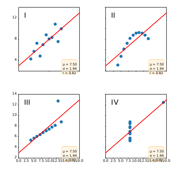
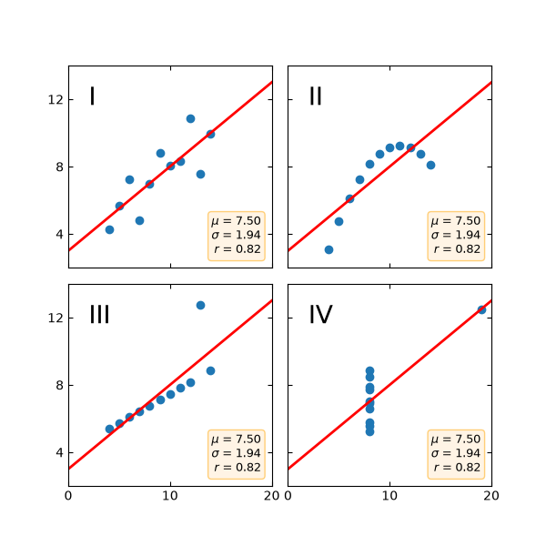
specialty_plots/hinton_demo
===============
Source
"""
===============
Hinton diagrams
===============
Hinton diagrams are useful for visualizing the values of a 2D array (e.g.
a weight matrix): Positive and negative values are represented by white and
black squares, respectively, and the size of each square represents the
magnitude of each value.
Initial idea from David Warde-Farley on the SciPy Cookbook
"""
import matplotlib.pyplot as plt
import numpy as np
def hinton(matrix, max_weight=None, ax=None):
"""Draw Hinton diagram for visualizing a weight matrix."""
ax = ax if ax is not None else plt.gca()
if not max_weight:
max_weight = 2 ** np.ceil(np.log2(np.abs(matrix).max()))
ax.patch.set_facecolor('gray')
ax.set_aspect('equal', 'box')
ax.xaxis.set_major_locator(plt.NullLocator())
ax.yaxis.set_major_locator(plt.NullLocator())
for (x, y), w in np.ndenumerate(matrix):
color = 'white' if w > 0 else 'black'
size = np.sqrt(abs(w) / max_weight)
rect = plt.Rectangle([x - size / 2, y - size / 2], size, size,
facecolor=color, edgecolor=color)
ax.add_patch(rect)
ax.autoscale_view()
ax.invert_yaxis()
if __name__ == '__main__':
# Fixing random state for reproducibility
np.random.seed(19680801)
hinton(np.random.rand(20, 20) - 0.5)
plt.show()
specialty_plots/ishikawa_diagram
================
Source
"""
================
Ishikawa Diagram
================
Ishikawa Diagrams, fishbone diagrams, herringbone diagrams, or cause-and-effect
diagrams are used to identify problems in a system by showing how causes and
effects are linked.
Source: https://en.wikipedia.org/wiki/Ishikawa_diagram
"""
import math
import matplotlib.pyplot as plt
from matplotlib.patches import Polygon, Wedge
fig, ax = plt.subplots(figsize=(10, 6), layout='constrained')
ax.set_xlim(-5, 5)
ax.set_ylim(-5, 5)
ax.axis('off')
def problems(data: str,
problem_x: float, problem_y: float,
angle_x: float, angle_y: float):
"""
Draw each problem section of the Ishikawa plot.
Parameters
----------
data : str
The name of the problem category.
problem_x, problem_y : float, optional
The `X` and `Y` positions of the problem arrows (`Y` defaults to zero).
angle_x, angle_y : float, optional
The angle of the problem annotations. They are always angled towards
the tail of the plot.
Returns
-------
None.
"""
ax.annotate(str.upper(data), xy=(problem_x, problem_y),
xytext=(angle_x, angle_y),
fontsize=10,
color='white',
weight='bold',
xycoords='data',
verticalalignment='center',
horizontalalignment='center',
textcoords='offset fontsize',
arrowprops=dict(arrowstyle="->", facecolor='black'),
bbox=dict(boxstyle='square',
facecolor='tab:blue',
pad=0.8))
def causes(data: list,
cause_x: float, cause_y: float,
cause_xytext=(-9, -0.3), top: bool = True):
"""
Place each cause to a position relative to the problems
annotations.
Parameters
----------
data : indexable object
The input data. IndexError is
raised if more than six arguments are passed.
cause_x, cause_y : float
The `X` and `Y` position of the cause annotations.
cause_xytext : tuple, optional
Adjust to set the distance of the cause text from the problem
arrow in fontsize units.
top : bool, default: True
Determines whether the next cause annotation will be
plotted above or below the previous one.
Returns
-------
None.
"""
for index, cause in enumerate(data):
# [<x pos>, <y pos>]
coords = [[0.02, 0],
[0.23, 0.5],
[-0.46, -1],
[0.69, 1.5],
[-0.92, -2],
[1.15, 2.5]]
# First 'cause' annotation is placed in the middle of the 'problems' arrow
# and each subsequent cause is plotted above or below it in succession.
cause_x -= coords[index][0]
cause_y += coords[index][1] if top else -coords[index][1]
ax.annotate(cause, xy=(cause_x, cause_y),
horizontalalignment='center',
xytext=cause_xytext,
fontsize=9,
xycoords='data',
textcoords='offset fontsize',
arrowprops=dict(arrowstyle="->",
facecolor='black'))
def draw_body(data: dict):
"""
Place each problem section in its correct place by changing
the coordinates on each loop.
Parameters
----------
data : dict
The input data (can be a dict of lists or tuples). ValueError
is raised if more than six arguments are passed.
Returns
-------
None.
"""
# Set the length of the spine according to the number of 'problem' categories.
length = (math.ceil(len(data) / 2)) - 1
draw_spine(-2 - length, 2 + length)
# Change the coordinates of the 'problem' annotations after each one is rendered.
offset = 0
prob_section = [1.55, 0.8]
for index, problem in enumerate(data.values()):
plot_above = index % 2 == 0
cause_arrow_y = 1.7 if plot_above else -1.7
y_prob_angle = 16 if plot_above else -16
# Plot each section in pairs along the main spine.
prob_arrow_x = prob_section[0] + length + offset
cause_arrow_x = prob_section[1] + length + offset
if not plot_above:
offset -= 2.5
if index > 5:
raise ValueError(f'Maximum number of problems is 6, you have entered '
f'{len(data)}')
problems(list(data.keys())[index], prob_arrow_x, 0, -12, y_prob_angle)
causes(problem, cause_arrow_x, cause_arrow_y, top=plot_above)
def draw_spine(xmin: int, xmax: int):
"""
Draw main spine, head and tail.
Parameters
----------
xmin : int
The default position of the head of the spine's
x-coordinate.
xmax : int
The default position of the tail of the spine's
x-coordinate.
Returns
-------
None.
"""
# draw main spine
ax.plot([xmin - 0.1, xmax], [0, 0], color='tab:blue', linewidth=2)
# draw fish head
ax.text(xmax + 0.1, - 0.05, 'PROBLEM', fontsize=10,
weight='bold', color='white')
semicircle = Wedge((xmax, 0), 1, 270, 90, fc='tab:blue')
ax.add_patch(semicircle)
# draw fish tail
tail_pos = [[xmin - 0.8, 0.8], [xmin - 0.8, -0.8], [xmin, -0.01]]
triangle = Polygon(tail_pos, fc='tab:blue')
ax.add_patch(triangle)
# Input data
categories = {
'Method': ['Time consumption', 'Cost', 'Procedures', 'Inefficient process',
'Sampling'],
'Machine': ['Faulty equipment', 'Compatibility'],
'Material': ['Poor-quality input', 'Raw materials', 'Supplier',
'Shortage'],
'Measurement': ['Calibration', 'Performance', 'Wrong measurements'],
'Environment': ['Bad conditions'],
'People': ['Lack of training', 'Managers', 'Labor shortage',
'Procedures', 'Sales strategy']
}
draw_body(categories)
plt.show()
specialty_plots/leftventricle_bullseye
=======================
Source
"""
=======================
Left ventricle bullseye
=======================
This example demonstrates how to create the 17 segment model for the left
ventricle recommended by the American Heart Association (AHA).
.. redirect-from:: /gallery/specialty_plots/leftventricle_bulleye
See also the :doc:`/gallery/pie_and_polar_charts/nested_pie` example.
"""
import matplotlib.pyplot as plt
import numpy as np
import matplotlib as mpl
def bullseye_plot(ax, data, seg_bold=None, cmap="viridis", norm=None):
"""
Bullseye representation for the left ventricle.
Parameters
----------
ax : Axes
data : list[float]
The intensity values for each of the 17 segments.
seg_bold : list[int], optional
A list with the segments to highlight.
cmap : colormap, default: "viridis"
Colormap for the data.
norm : Normalize or None, optional
Normalizer for the data.
Notes
-----
This function creates the 17 segment model for the left ventricle according
to the American Heart Association (AHA) [1]_
References
----------
.. [1] M. D. Cerqueira, N. J. Weissman, V. Dilsizian, A. K. Jacobs,
S. Kaul, W. K. Laskey, D. J. Pennell, J. A. Rumberger, T. Ryan,
and M. S. Verani, "Standardized myocardial segmentation and
nomenclature for tomographic imaging of the heart",
Circulation, vol. 105, no. 4, pp. 539-542, 2002.
"""
data = np.ravel(data)
if seg_bold is None:
seg_bold = []
if norm is None:
norm = mpl.colors.Normalize(vmin=data.min(), vmax=data.max())
r = np.linspace(0.2, 1, 4)
ax.set(ylim=(0, 1), xticklabels=[], yticklabels=[])
ax.grid(False) # Remove grid
# Fill segments 1-6, 7-12, 13-16.
for start, stop, r_in, r_out in [
(0, 6, r[2], r[3]),
(6, 12, r[1], r[2]),
(12, 16, r[0], r[1]),
(16, 17, 0, r[0]),
]:
n = stop - start
dtheta = 2*np.pi / n
ax.bar(np.arange(n) * dtheta + np.pi/2, r_out - r_in, dtheta, r_in,
color=cmap(norm(data[start:stop])))
# Now, draw the segment borders. In order for the outer bold borders not
# to be covered by inner segments, the borders are all drawn separately
# after the segments have all been filled. We also disable clipping, which
# would otherwise affect the outermost segment edges.
# Draw edges of segments 1-6, 7-12, 13-16.
for start, stop, r_in, r_out in [
(0, 6, r[2], r[3]),
(6, 12, r[1], r[2]),
(12, 16, r[0], r[1]),
]:
n = stop - start
dtheta = 2*np.pi / n
ax.bar(np.arange(n) * dtheta + np.pi/2, r_out - r_in, dtheta, r_in,
clip_on=False, color="none", edgecolor="k", linewidth=[
4 if i + 1 in seg_bold else 2 for i in range(start, stop)])
# Draw edge of segment 17 -- here; the edge needs to be drawn differently,
# using plot().
ax.plot(np.linspace(0, 2*np.pi), np.linspace(r[0], r[0]), "k",
linewidth=(4 if 17 in seg_bold else 2))
# Create the fake data
data = np.arange(17) + 1
# Make a figure and Axes with dimensions as desired.
fig = plt.figure(figsize=(10, 5), layout="constrained")
fig.get_layout_engine().set(wspace=.1, w_pad=.2)
axs = fig.subplots(1, 3, subplot_kw=dict(projection='polar'))
fig.canvas.manager.set_window_title('Left Ventricle Bulls Eyes (AHA)')
# Set the colormap and norm to correspond to the data for which
# the colorbar will be used.
cmap = mpl.colormaps["viridis"]
norm = mpl.colors.Normalize(vmin=1, vmax=17)
# Create an empty ScalarMappable to set the colorbar's colormap and norm.
# The following gives a basic continuous colorbar with ticks and labels.
fig.colorbar(mpl.cm.ScalarMappable(cmap=cmap, norm=norm),
cax=axs[0].inset_axes([0, -.15, 1, .1]),
orientation='horizontal', label='Some units')
# And again for the second colorbar.
cmap2 = mpl.colormaps["cool"]
norm2 = mpl.colors.Normalize(vmin=1, vmax=17)
fig.colorbar(mpl.cm.ScalarMappable(cmap=cmap2, norm=norm2),
cax=axs[1].inset_axes([0, -.15, 1, .1]),
orientation='horizontal', label='Some other units')
# The second example illustrates the use of a ListedColormap, a
# BoundaryNorm, and extended ends to show the "over" and "under"
# value colors.
cmap3 = mpl.colors.ListedColormap(['r', 'g', 'b', 'c'], over='0.35', under='0.75')
# If a ListedColormap is used, the length of the bounds array must be
# one greater than the length of the color list. The bounds must be
# monotonically increasing.
bounds = [2, 3, 7, 9, 15]
norm3 = mpl.colors.BoundaryNorm(bounds, cmap3.N)
fig.colorbar(mpl.cm.ScalarMappable(cmap=cmap3, norm=norm3),
cax=axs[2].inset_axes([0, -.15, 1, .1]),
extend='both',
ticks=bounds, # optional
spacing='proportional',
orientation='horizontal',
label='Discrete intervals, some other units')
# Create the 17 segment model
bullseye_plot(axs[0], data, cmap=cmap, norm=norm)
axs[0].set_title('Bulls Eye (AHA)')
bullseye_plot(axs[1], data, cmap=cmap2, norm=norm2)
axs[1].set_title('Bulls Eye (AHA)')
bullseye_plot(axs[2], data, seg_bold=[3, 5, 6, 11, 12, 16],
cmap=cmap3, norm=norm3)
axs[2].set_title('Segments [3, 5, 6, 11, 12, 16] in bold')
plt.show()
specialty_plots/mri_with_eeg
============
Source
"""
============
MRI with EEG
============
Displays a set of subplots with an MRI image, its intensity
histogram and some EEG traces.
.. redirect-from:: /gallery/specialty_plots/mri_demo
"""
import matplotlib.pyplot as plt
import numpy as np
import matplotlib.cbook as cbook
fig, axd = plt.subplot_mosaic(
[["image", "density"],
["EEG", "EEG"]],
layout="constrained",
# "image" will contain a square image. We fine-tune the width so that
# there is no excess horizontal or vertical margin around the image.
width_ratios=[1.05, 2],
)
# Load the MRI data (256x256 16-bit integers)
with cbook.get_sample_data('s1045.ima.gz') as dfile:
im = np.frombuffer(dfile.read(), np.uint16).reshape((256, 256))
# Plot the MRI image
axd["image"].imshow(im, cmap="gray")
axd["image"].axis('off')
# Plot the histogram of MRI intensity
im = im[im.nonzero()] # Ignore the background
axd["density"].hist(im, bins=np.arange(0, 2**16+1, 512))
axd["density"].set(xlabel='Intensity (a.u.)', xlim=(0, 2**16),
ylabel='MRI density', yticks=[])
axd["density"].minorticks_on()
# Load the EEG data
n_samples, n_rows = 800, 4
with cbook.get_sample_data('eeg.dat') as eegfile:
data = np.fromfile(eegfile, dtype=float).reshape((n_samples, n_rows))
t = 10 * np.arange(n_samples) / n_samples
# Plot the EEG
axd["EEG"].set_xlabel('Time (s)')
axd["EEG"].set_xlim(0, 10)
dy = (data.min() - data.max()) * 0.7 # Crowd them a bit.
axd["EEG"].set_ylim(-dy, n_rows * dy)
axd["EEG"].set_yticks([0, dy, 2*dy, 3*dy], labels=['PG3', 'PG5', 'PG7', 'PG9'])
for i, data_col in enumerate(data.T):
axd["EEG"].plot(t, data_col + i*dy, color="C0")
plt.show()
specialty_plots/radar_chart
======================================
Source
"""
======================================
Radar chart (aka spider or star chart)
======================================
This example creates a radar chart, also known as a spider or star chart [1]_.
Although this example allows a frame of either 'circle' or 'polygon', polygon
frames don't have proper gridlines (the lines are circles instead of polygons).
It's possible to get a polygon grid by setting GRIDLINE_INTERPOLATION_STEPS in
`matplotlib.axis` to the desired number of vertices, but the orientation of the
polygon is not aligned with the radial axis.
.. [1] https://en.wikipedia.org/wiki/Radar_chart
"""
import matplotlib.pyplot as plt
import numpy as np
from matplotlib.patches import Circle, RegularPolygon
from matplotlib.path import Path
from matplotlib.projections import register_projection
from matplotlib.projections.polar import PolarAxes
from matplotlib.spines import Spine
from matplotlib.transforms import Affine2D
def radar_factory(num_vars, frame='circle'):
"""
Create a radar chart with `num_vars` Axes.
This function creates a RadarAxes projection and registers it.
Parameters
----------
num_vars : int
Number of variables for radar chart.
frame : {'circle', 'polygon'}
Shape of frame surrounding Axes.
"""
# calculate evenly-spaced axis angles
theta = np.linspace(0, 2*np.pi, num_vars, endpoint=False)
class RadarTransform(PolarAxes.PolarTransform):
def transform_path_non_affine(self, path):
# Paths with non-unit interpolation steps correspond to gridlines,
# in which case we force interpolation (to defeat PolarTransform's
# autoconversion to circular arcs).
if path._interpolation_steps > 1:
path = path.interpolated(num_vars)
return Path(self.transform(path.vertices), path.codes)
class RadarAxes(PolarAxes):
name = 'radar'
PolarTransform = RadarTransform
def __init__(self, *args, **kwargs):
super().__init__(*args, **kwargs)
# rotate plot such that the first axis is at the top
self.set_theta_zero_location('N')
def fill(self, *args, closed=True, **kwargs):
"""Override fill so that line is closed by default"""
return super().fill(closed=closed, *args, **kwargs)
def plot(self, *args, **kwargs):
"""Override plot so that line is closed by default"""
lines = super().plot(*args, **kwargs)
for line in lines:
self._close_line(line)
def _close_line(self, line):
x, y = line.get_data()
# FIXME: markers at x[0], y[0] get doubled-up
if x[0] != x[-1]:
x = np.append(x, x[0])
y = np.append(y, y[0])
line.set_data(x, y)
def set_varlabels(self, labels):
self.set_thetagrids(np.degrees(theta), labels)
def _gen_axes_patch(self):
# The Axes patch must be centered at (0.5, 0.5) and of radius 0.5
# in axes coordinates.
if frame == 'circle':
return Circle((0.5, 0.5), 0.5)
elif frame == 'polygon':
return RegularPolygon((0.5, 0.5), num_vars,
radius=.5, edgecolor="k")
else:
raise ValueError("Unknown value for 'frame': %s" % frame)
def _gen_axes_spines(self):
if frame == 'circle':
return super()._gen_axes_spines()
elif frame == 'polygon':
# spine_type must be 'left'/'right'/'top'/'bottom'/'circle'.
spine = Spine(axes=self,
spine_type='circle',
path=Path.unit_regular_polygon(num_vars))
# unit_regular_polygon gives a polygon of radius 1 centered at
# (0, 0) but we want a polygon of radius 0.5 centered at (0.5,
# 0.5) in axes coordinates.
spine.set_transform(Affine2D().scale(.5).translate(.5, .5)
+ self.transAxes)
return {'polar': spine}
else:
raise ValueError("Unknown value for 'frame': %s" % frame)
register_projection(RadarAxes)
return theta
def example_data():
# The following data is from the Denver Aerosol Sources and Health study.
# See doi:10.1016/j.atmosenv.2008.12.017
#
# The data are pollution source profile estimates for five modeled
# pollution sources (e.g., cars, wood-burning, etc) that emit 7-9 chemical
# species. The radar charts are experimented with here to see if we can
# nicely visualize how the modeled source profiles change across four
# scenarios:
# 1) No gas-phase species present, just seven particulate counts on
# Sulfate
# Nitrate
# Elemental Carbon (EC)
# Organic Carbon fraction 1 (OC)
# Organic Carbon fraction 2 (OC2)
# Organic Carbon fraction 3 (OC3)
# Pyrolyzed Organic Carbon (OP)
# 2)Inclusion of gas-phase specie carbon monoxide (CO)
# 3)Inclusion of gas-phase specie ozone (O3).
# 4)Inclusion of both gas-phase species is present...
data = [
['Sulfate', 'Nitrate', 'EC', 'OC1', 'OC2', 'OC3', 'OP', 'CO', 'O3'],
('Basecase', [
[0.88, 0.01, 0.03, 0.03, 0.00, 0.06, 0.01, 0.00, 0.00],
[0.07, 0.95, 0.04, 0.05, 0.00, 0.02, 0.01, 0.00, 0.00],
[0.01, 0.02, 0.85, 0.19, 0.05, 0.10, 0.00, 0.00, 0.00],
[0.02, 0.01, 0.07, 0.01, 0.21, 0.12, 0.98, 0.00, 0.00],
[0.01, 0.01, 0.02, 0.71, 0.74, 0.70, 0.00, 0.00, 0.00]]),
('With CO', [
[0.88, 0.02, 0.02, 0.02, 0.00, 0.05, 0.00, 0.05, 0.00],
[0.08, 0.94, 0.04, 0.02, 0.00, 0.01, 0.12, 0.04, 0.00],
[0.01, 0.01, 0.79, 0.10, 0.00, 0.05, 0.00, 0.31, 0.00],
[0.00, 0.02, 0.03, 0.38, 0.31, 0.31, 0.00, 0.59, 0.00],
[0.02, 0.02, 0.11, 0.47, 0.69, 0.58, 0.88, 0.00, 0.00]]),
('With O3', [
[0.89, 0.01, 0.07, 0.00, 0.00, 0.05, 0.00, 0.00, 0.03],
[0.07, 0.95, 0.05, 0.04, 0.00, 0.02, 0.12, 0.00, 0.00],
[0.01, 0.02, 0.86, 0.27, 0.16, 0.19, 0.00, 0.00, 0.00],
[0.01, 0.03, 0.00, 0.32, 0.29, 0.27, 0.00, 0.00, 0.95],
[0.02, 0.00, 0.03, 0.37, 0.56, 0.47, 0.87, 0.00, 0.00]]),
('CO & O3', [
[0.87, 0.01, 0.08, 0.00, 0.00, 0.04, 0.00, 0.00, 0.01],
[0.09, 0.95, 0.02, 0.03, 0.00, 0.01, 0.13, 0.06, 0.00],
[0.01, 0.02, 0.71, 0.24, 0.13, 0.16, 0.00, 0.50, 0.00],
[0.01, 0.03, 0.00, 0.28, 0.24, 0.23, 0.00, 0.44, 0.88],
[0.02, 0.00, 0.18, 0.45, 0.64, 0.55, 0.86, 0.00, 0.16]])
]
return data
if __name__ == '__main__':
N = 9
theta = radar_factory(N, frame='polygon')
data = example_data()
spoke_labels = data.pop(0)
fig, axs = plt.subplots(figsize=(9, 9), nrows=2, ncols=2,
subplot_kw=dict(projection='radar'))
fig.subplots_adjust(wspace=0.25, hspace=0.20, top=0.85, bottom=0.05)
colors = ['b', 'r', 'g', 'm', 'y']
# Plot the four cases from the example data on separate Axes
for ax, (title, case_data) in zip(axs.flat, data):
ax.set_rgrids([0.2, 0.4, 0.6, 0.8])
ax.set_title(title, weight='bold', size='medium', position=(0.5, 1.1),
horizontalalignment='center', verticalalignment='center')
for d, color in zip(case_data, colors):
ax.plot(theta, d, color=color)
ax.fill(theta, d, facecolor=color, alpha=0.25, label='_nolegend_')
ax.set_varlabels(spoke_labels)
# add legend relative to top-left plot
labels = ('Factor 1', 'Factor 2', 'Factor 3', 'Factor 4', 'Factor 5')
legend = axs[0, 0].legend(labels, loc=(0.9, .95),
labelspacing=0.1, fontsize='small')
fig.text(0.5, 0.965, '5-Factor Solution Profiles Across Four Scenarios',
horizontalalignment='center', color='black', weight='bold',
size='large')
plt.show()
# %%
#
# .. admonition:: References
#
# The use of the following functions, methods, classes and modules is shown
# in this example:
#
# - `matplotlib.path`
# - `matplotlib.path.Path`
# - `matplotlib.spines`
# - `matplotlib.spines.Spine`
# - `matplotlib.projections`
# - `matplotlib.projections.polar`
# - `matplotlib.projections.polar.PolarAxes`
# - `matplotlib.projections.register_projection`
AttributeError: 'Axes' object has no attribute 'set_varlabels'
specialty_plots/sankey_basics
================
Source
"""
================
The Sankey class
================
Demonstrate the Sankey class by producing three basic diagrams.
"""
import matplotlib.pyplot as plt
from matplotlib.sankey import Sankey
# %%
# Example 1 -- Mostly defaults
#
# This demonstrates how to create a simple diagram by implicitly calling the
# Sankey.add() method and by appending finish() to the call to the class.
Sankey(flows=[0.25, 0.15, 0.60, -0.20, -0.15, -0.05, -0.50, -0.10],
labels=['', '', '', 'First', 'Second', 'Third', 'Fourth', 'Fifth'],
orientations=[-1, 1, 0, 1, 1, 1, 0, -1]).finish()
plt.title("The default settings produce a diagram like this.")
# %%
# Notice:
#
# 1. Axes weren't provided when Sankey() was instantiated, so they were
# created automatically.
# 2. The scale argument wasn't necessary since the data was already
# normalized.
# 3. By default, the lengths of the paths are justified.
# %%
# Example 2
#
# This demonstrates:
#
# 1. Setting one path longer than the others
# 2. Placing a label in the middle of the diagram
# 3. Using the scale argument to normalize the flows
# 4. Implicitly passing keyword arguments to PathPatch()
# 5. Changing the angle of the arrow heads
# 6. Changing the offset between the tips of the paths and their labels
# 7. Formatting the numbers in the path labels and the associated unit
# 8. Changing the appearance of the patch and the labels after the figure is
# created
fig = plt.figure()
ax = fig.add_subplot(1, 1, 1, xticks=[], yticks=[],
title="Flow Diagram of a Widget")
sankey = Sankey(ax=ax, scale=0.01, offset=0.2, head_angle=180,
format='%.0f', unit='%')
sankey.add(flows=[25, 0, 60, -10, -20, -5, -15, -10, -40],
labels=['', '', '', 'First', 'Second', 'Third', 'Fourth',
'Fifth', 'Hurray!'],
orientations=[-1, 1, 0, 1, 1, 1, -1, -1, 0],
pathlengths=[0.25, 0.25, 0.25, 0.25, 0.25, 0.6, 0.25, 0.25,
0.25],
patchlabel="Widget\nA") # Arguments to matplotlib.patches.PathPatch
diagrams = sankey.finish()
diagrams[0].texts[-1].set_color('r')
diagrams[0].text.set_fontweight('bold')
# %%
# Notice:
#
# 1. Since the sum of the flows is nonzero, the width of the trunk isn't
# uniform. The matplotlib logging system logs this at the DEBUG level.
# 2. The second flow doesn't appear because its value is zero. Again, this is
# logged at the DEBUG level.
# %%
# Example 3
#
# This demonstrates:
#
# 1. Connecting two systems
# 2. Turning off the labels of the quantities
# 3. Adding a legend
fig = plt.figure()
ax = fig.add_subplot(1, 1, 1, xticks=[], yticks=[], title="Two Systems")
flows = [0.25, 0.15, 0.60, -0.10, -0.05, -0.25, -0.15, -0.10, -0.35]
sankey = Sankey(ax=ax, unit=None)
sankey.add(flows=flows, label='one',
orientations=[-1, 1, 0, 1, 1, 1, -1, -1, 0])
sankey.add(flows=[-0.25, 0.15, 0.1], label='two',
orientations=[-1, -1, -1], prior=0, connect=(0, 0))
diagrams = sankey.finish()
diagrams[-1].patch.set_hatch('/')
plt.legend()
# %%
# Notice that only one connection is specified, but the systems form a
# circuit since: (1) the lengths of the paths are justified and (2) the
# orientation and ordering of the flows is mirrored.
plt.show()
# %%
#
# .. admonition:: References
#
# The use of the following functions, methods, classes and modules is shown
# in this example:
#
# - `matplotlib.sankey`
# - `matplotlib.sankey.Sankey`
# - `matplotlib.sankey.Sankey.add`
# - `matplotlib.sankey.Sankey.finish`
specialty_plots/sankey_links
======================================
Source
"""
======================================
Long chain of connections using Sankey
======================================
Demonstrate/test the Sankey class by producing a long chain of connections.
"""
import matplotlib.pyplot as plt
from matplotlib.sankey import Sankey
links_per_side = 6
def side(sankey, n=1):
"""Generate a side chain."""
prior = len(sankey.diagrams)
for i in range(0, 2*n, 2):
sankey.add(flows=[1, -1], orientations=[-1, -1],
patchlabel=str(prior + i),
prior=prior + i - 1, connect=(1, 0), alpha=0.5)
sankey.add(flows=[1, -1], orientations=[1, 1],
patchlabel=str(prior + i + 1),
prior=prior + i, connect=(1, 0), alpha=0.5)
def corner(sankey):
"""Generate a corner link."""
prior = len(sankey.diagrams)
sankey.add(flows=[1, -1], orientations=[0, 1],
patchlabel=str(prior), facecolor='k',
prior=prior - 1, connect=(1, 0), alpha=0.5)
fig = plt.figure()
ax = fig.add_subplot(1, 1, 1, xticks=[], yticks=[],
title="Why would you want to do this?\n(But you could.)")
sankey = Sankey(ax=ax, unit=None)
sankey.add(flows=[1, -1], orientations=[0, 1],
patchlabel="0", facecolor='k',
rotation=45)
side(sankey, n=links_per_side)
corner(sankey)
side(sankey, n=links_per_side)
corner(sankey)
side(sankey, n=links_per_side)
corner(sankey)
side(sankey, n=links_per_side)
sankey.finish()
# Notice:
# 1. The alignment doesn't drift significantly (if at all; with 16007
# subdiagrams there is still closure).
# 2. The first diagram is rotated 45 deg, so all other diagrams are rotated
# accordingly.
plt.show()
# %%
#
# .. admonition:: References
#
# The use of the following functions, methods, classes and modules is shown
# in this example:
#
# - `matplotlib.sankey`
# - `matplotlib.sankey.Sankey`
# - `matplotlib.sankey.Sankey.add`
# - `matplotlib.sankey.Sankey.finish`
specialty_plots/sankey_rankine
===================
Source
"""
===================
Rankine power cycle
===================
Demonstrate the Sankey class with a practical example of a Rankine power cycle.
"""
import matplotlib.pyplot as plt
from matplotlib.sankey import Sankey
fig = plt.figure(figsize=(8, 9))
ax = fig.add_subplot(1, 1, 1, xticks=[], yticks=[],
title="Rankine Power Cycle: Example 8.6 from Moran and "
"Shapiro\n\x22Fundamentals of Engineering Thermodynamics "
"\x22, 6th ed., 2008")
Hdot = [260.431, 35.078, 180.794, 221.115, 22.700,
142.361, 10.193, 10.210, 43.670, 44.312,
68.631, 10.758, 10.758, 0.017, 0.642,
232.121, 44.559, 100.613, 132.168] # MW
sankey = Sankey(ax=ax, format='%.3G', unit=' MW', gap=0.5, scale=1.0/Hdot[0])
sankey.add(patchlabel='\n\nPump 1', rotation=90, facecolor='#37c959',
flows=[Hdot[13], Hdot[6], -Hdot[7]],
labels=['Shaft power', '', None],
pathlengths=[0.4, 0.883, 0.25],
orientations=[1, -1, 0])
sankey.add(patchlabel='\n\nOpen\nheater', facecolor='#37c959',
flows=[Hdot[11], Hdot[7], Hdot[4], -Hdot[8]],
labels=[None, '', None, None],
pathlengths=[0.25, 0.25, 1.93, 0.25],
orientations=[1, 0, -1, 0], prior=0, connect=(2, 1))
sankey.add(patchlabel='\n\nPump 2', facecolor='#37c959',
flows=[Hdot[14], Hdot[8], -Hdot[9]],
labels=['Shaft power', '', None],
pathlengths=[0.4, 0.25, 0.25],
orientations=[1, 0, 0], prior=1, connect=(3, 1))
sankey.add(patchlabel='Closed\nheater', trunklength=2.914, fc='#37c959',
flows=[Hdot[9], Hdot[1], -Hdot[11], -Hdot[10]],
pathlengths=[0.25, 1.543, 0.25, 0.25],
labels=['', '', None, None],
orientations=[0, -1, 1, -1], prior=2, connect=(2, 0))
sankey.add(patchlabel='Trap', facecolor='#37c959', trunklength=5.102,
flows=[Hdot[11], -Hdot[12]],
labels=['\n', None],
pathlengths=[1.0, 1.01],
orientations=[1, 1], prior=3, connect=(2, 0))
sankey.add(patchlabel='Steam\ngenerator', facecolor='#ff5555',
flows=[Hdot[15], Hdot[10], Hdot[2], -Hdot[3], -Hdot[0]],
labels=['Heat rate', '', '', None, None],
pathlengths=0.25,
orientations=[1, 0, -1, -1, -1], prior=3, connect=(3, 1))
sankey.add(patchlabel='\n\n\nTurbine 1', facecolor='#37c959',
flows=[Hdot[0], -Hdot[16], -Hdot[1], -Hdot[2]],
labels=['', None, None, None],
pathlengths=[0.25, 0.153, 1.543, 0.25],
orientations=[0, 1, -1, -1], prior=5, connect=(4, 0))
sankey.add(patchlabel='\n\n\nReheat', facecolor='#37c959',
flows=[Hdot[2], -Hdot[2]],
labels=[None, None],
pathlengths=[0.725, 0.25],
orientations=[-1, 0], prior=6, connect=(3, 0))
sankey.add(patchlabel='Turbine 2', trunklength=3.212, facecolor='#37c959',
flows=[Hdot[3], Hdot[16], -Hdot[5], -Hdot[4], -Hdot[17]],
labels=[None, 'Shaft power', None, '', 'Shaft power'],
pathlengths=[0.751, 0.15, 0.25, 1.93, 0.25],
orientations=[0, -1, 0, -1, 1], prior=6, connect=(1, 1))
sankey.add(patchlabel='Condenser', facecolor='#58b1fa', trunklength=1.764,
flows=[Hdot[5], -Hdot[18], -Hdot[6]],
labels=['', 'Heat rate', None],
pathlengths=[0.45, 0.25, 0.883],
orientations=[-1, 1, 0], prior=8, connect=(2, 0))
diagrams = sankey.finish()
for diagram in diagrams:
diagram.text.set_fontweight('bold')
diagram.text.set_fontsize('10')
for text in diagram.texts:
text.set_fontsize('10')
# Notice that the explicit connections are handled automatically, but the
# implicit ones currently are not. The lengths of the paths and the trunks
# must be adjusted manually, and that is a bit tricky.
plt.show()
# %%
#
# .. admonition:: References
#
# The use of the following functions, methods, classes and modules is shown
# in this example:
#
# - `matplotlib.sankey`
# - `matplotlib.sankey.Sankey`
# - `matplotlib.sankey.Sankey.add`
# - `matplotlib.sankey.Sankey.finish`
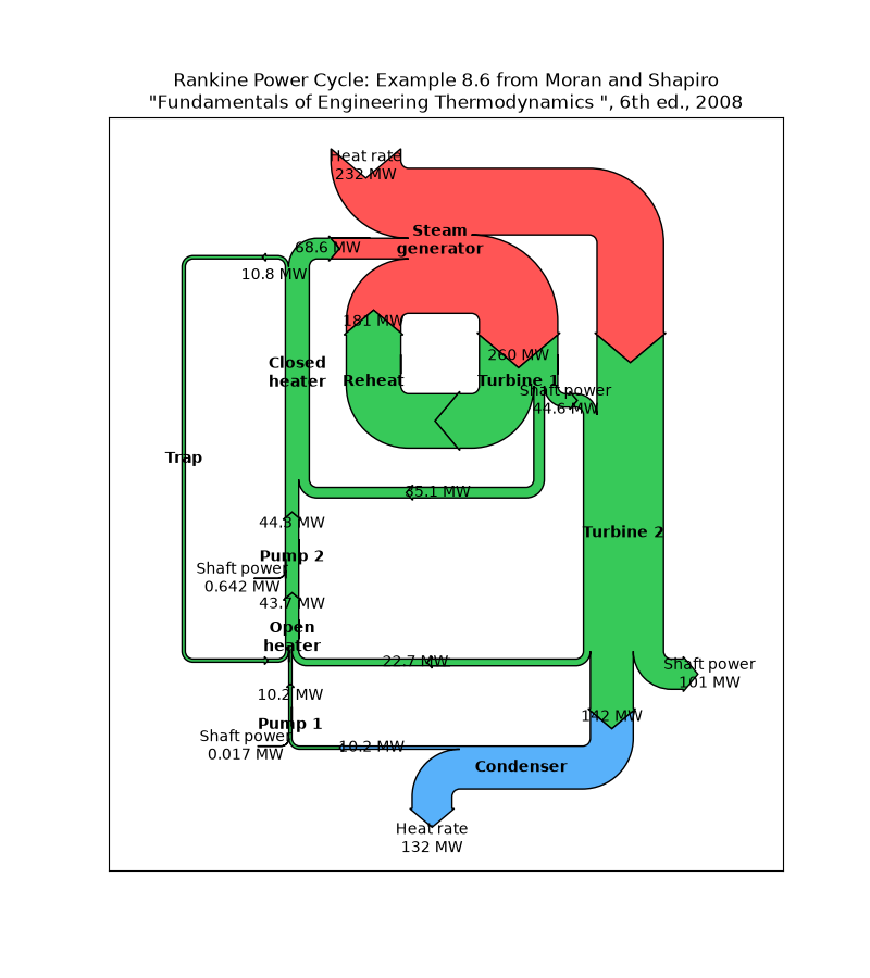
specialty_plots/skewt
===========================================================
Source
"""
===========================================================
SkewT-logP diagram: using transforms and custom projections
===========================================================
This serves as an intensive exercise of Matplotlib's transforms and custom
projection API. This example produces a so-called SkewT-logP diagram, which is
a common plot in meteorology for displaying vertical profiles of temperature.
As far as Matplotlib is concerned, the complexity comes from having X and Y
axes that are not orthogonal. This is handled by including a skew component to
the basic Axes transforms. Additional complexity comes in handling the fact
that the upper and lower X-axes have different data ranges, which necessitates
a bunch of custom classes for ticks, spines, and axis to handle this.
"""
from contextlib import ExitStack
from matplotlib.axes import Axes
import matplotlib.axis as maxis
from matplotlib.projections import register_projection
import matplotlib.spines as mspines
import matplotlib.transforms as transforms
# The sole purpose of this class is to look at the upper, lower, or total
# interval as appropriate and see what parts of the tick to draw, if any.
class SkewXTick(maxis.XTick):
def draw(self, renderer):
# When adding the callbacks with `stack.callback`, we fetch the current
# visibility state of the artist with `get_visible`; the ExitStack will
# restore these states (`set_visible`) at the end of the block (after
# the draw).
with ExitStack() as stack:
for artist in [self.gridline, self.tick1line, self.tick2line,
self.label1, self.label2]:
stack.callback(artist.set_visible, artist.get_visible())
needs_lower = transforms._interval_contains(
self.axes.lower_xlim, self.get_loc())
needs_upper = transforms._interval_contains(
self.axes.upper_xlim, self.get_loc())
self.tick1line.set_visible(
self.tick1line.get_visible() and needs_lower)
self.label1.set_visible(
self.label1.get_visible() and needs_lower)
self.tick2line.set_visible(
self.tick2line.get_visible() and needs_upper)
self.label2.set_visible(
self.label2.get_visible() and needs_upper)
super().draw(renderer)
def get_view_interval(self):
return self.axes.xaxis.get_view_interval()
# This class exists to provide two separate sets of intervals to the tick,
# as well as create instances of the custom tick
class SkewXAxis(maxis.XAxis):
def _get_tick(self, major):
return SkewXTick(self.axes, None, major=major)
def get_view_interval(self):
return self.axes.upper_xlim[0], self.axes.lower_xlim[1]
# This class exists to calculate the separate data range of the
# upper X-axis and draw the spine there. It also provides this range
# to the X-axis artist for ticking and gridlines
class SkewSpine(mspines.Spine):
def _adjust_location(self):
pts = self._path.vertices
if self.spine_type == 'top':
pts[:, 0] = self.axes.upper_xlim
else:
pts[:, 0] = self.axes.lower_xlim
# This class handles registration of the skew-xaxes as a projection as well
# as setting up the appropriate transformations. It also overrides standard
# spines and axes instances as appropriate.
class SkewXAxes(Axes):
# The projection must specify a name. This will be used be the
# user to select the projection, i.e. ``subplot(projection='skewx')``.
name = 'skewx'
def _init_axis(self):
# Taken from Axes and modified to use our modified X-axis
self.xaxis = SkewXAxis(self)
self.spines.top.register_axis(self.xaxis)
self.spines.bottom.register_axis(self.xaxis)
self.yaxis = maxis.YAxis(self)
self.spines.left.register_axis(self.yaxis)
self.spines.right.register_axis(self.yaxis)
def _gen_axes_spines(self):
spines = {'top': SkewSpine.linear_spine(self, 'top'),
'bottom': mspines.Spine.linear_spine(self, 'bottom'),
'left': mspines.Spine.linear_spine(self, 'left'),
'right': mspines.Spine.linear_spine(self, 'right')}
return spines
def _set_lim_and_transforms(self):
"""
This is called once when the plot is created to set up all the
transforms for the data, text and grids.
"""
rot = 30
# Get the standard transform setup from the Axes base class
super()._set_lim_and_transforms()
# Need to put the skew in the middle, after the scale and limits,
# but before the transAxes. This way, the skew is done in Axes
# coordinates thus performing the transform around the proper origin
# We keep the pre-transAxes transform around for other users, like the
# spines for finding bounds
self.transDataToAxes = (
self.transScale
+ self.transLimits
+ transforms.Affine2D().skew_deg(rot, 0)
)
# Create the full transform from Data to Pixels
self.transData = self.transDataToAxes + self.transAxes
# Blended transforms like this need to have the skewing applied using
# both axes, in axes coords like before.
self._xaxis_transform = (
transforms.blended_transform_factory(
self.transScale + self.transLimits,
transforms.IdentityTransform())
+ transforms.Affine2D().skew_deg(rot, 0)
+ self.transAxes
)
@property
def lower_xlim(self):
return self.axes.viewLim.intervalx
@property
def upper_xlim(self):
pts = [[0., 1.], [1., 1.]]
return self.transDataToAxes.inverted().transform(pts)[:, 0]
# Now register the projection with matplotlib so the user can select it.
register_projection(SkewXAxes)
if __name__ == '__main__':
# Now make a simple example using the custom projection.
from io import StringIO
import matplotlib.pyplot as plt
import numpy as np
from matplotlib.ticker import MultipleLocator, NullFormatter, ScalarFormatter
# Some example data.
data_txt = '''
978.0 345 7.8 0.8
971.0 404 7.2 0.2
946.7 610 5.2 -1.8
944.0 634 5.0 -2.0
925.0 798 3.4 -2.6
911.8 914 2.4 -2.7
906.0 966 2.0 -2.7
877.9 1219 0.4 -3.2
850.0 1478 -1.3 -3.7
841.0 1563 -1.9 -3.8
823.0 1736 1.4 -0.7
813.6 1829 4.5 1.2
809.0 1875 6.0 2.2
798.0 1988 7.4 -0.6
791.0 2061 7.6 -1.4
783.9 2134 7.0 -1.7
755.1 2438 4.8 -3.1
727.3 2743 2.5 -4.4
700.5 3048 0.2 -5.8
700.0 3054 0.2 -5.8
698.0 3077 0.0 -6.0
687.0 3204 -0.1 -7.1
648.9 3658 -3.2 -10.9
631.0 3881 -4.7 -12.7
600.7 4267 -6.4 -16.7
592.0 4381 -6.9 -17.9
577.6 4572 -8.1 -19.6
555.3 4877 -10.0 -22.3
536.0 5151 -11.7 -24.7
533.8 5182 -11.9 -25.0
500.0 5680 -15.9 -29.9
472.3 6096 -19.7 -33.4
453.0 6401 -22.4 -36.0
400.0 7310 -30.7 -43.7
399.7 7315 -30.8 -43.8
387.0 7543 -33.1 -46.1
382.7 7620 -33.8 -46.8
342.0 8398 -40.5 -53.5
320.4 8839 -43.7 -56.7
318.0 8890 -44.1 -57.1
310.0 9060 -44.7 -58.7
306.1 9144 -43.9 -57.9
305.0 9169 -43.7 -57.7
300.0 9280 -43.5 -57.5
292.0 9462 -43.7 -58.7
276.0 9838 -47.1 -62.1
264.0 10132 -47.5 -62.5
251.0 10464 -49.7 -64.7
250.0 10490 -49.7 -64.7
247.0 10569 -48.7 -63.7
244.0 10649 -48.9 -63.9
243.3 10668 -48.9 -63.9
220.0 11327 -50.3 -65.3
212.0 11569 -50.5 -65.5
210.0 11631 -49.7 -64.7
200.0 11950 -49.9 -64.9
194.0 12149 -49.9 -64.9
183.0 12529 -51.3 -66.3
164.0 13233 -55.3 -68.3
152.0 13716 -56.5 -69.5
150.0 13800 -57.1 -70.1
136.0 14414 -60.5 -72.5
132.0 14600 -60.1 -72.1
131.4 14630 -60.2 -72.2
128.0 14792 -60.9 -72.9
125.0 14939 -60.1 -72.1
119.0 15240 -62.2 -73.8
112.0 15616 -64.9 -75.9
108.0 15838 -64.1 -75.1
107.8 15850 -64.1 -75.1
105.0 16010 -64.7 -75.7
103.0 16128 -62.9 -73.9
100.0 16310 -62.5 -73.5
'''
# Parse the data
sound_data = StringIO(data_txt)
p, h, T, Td = np.loadtxt(sound_data, unpack=True)
# Create a new figure. The dimensions here give a good aspect ratio
fig = plt.figure(figsize=(6.5875, 6.2125))
ax = fig.add_subplot(projection='skewx')
plt.grid(True)
# Plot the data using normal plotting functions, in this case using
# log scaling in Y, as dictated by the typical meteorological plot
ax.semilogy(T, p, color='C3')
ax.semilogy(Td, p, color='C2')
# An example of a slanted line at constant X
l = ax.axvline(0, color='C0')
# Disables the log-formatting that comes with semilogy
ax.yaxis.set_major_formatter(ScalarFormatter())
ax.yaxis.set_minor_formatter(NullFormatter())
ax.set_yticks(np.linspace(100, 1000, 10))
ax.set_ylim(1050, 100)
ax.xaxis.set_major_locator(MultipleLocator(10))
ax.set_xlim(-50, 50)
plt.show()
# %%
#
# .. admonition:: References
#
# The use of the following functions, methods, classes and modules is shown
# in this example:
#
# - `matplotlib.transforms`
# - `matplotlib.spines`
# - `matplotlib.spines.Spine`
# - `matplotlib.spines.Spine.register_axis`
# - `matplotlib.projections`
# - `matplotlib.projections.register_projection`
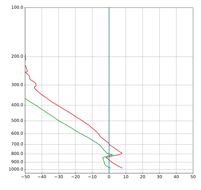
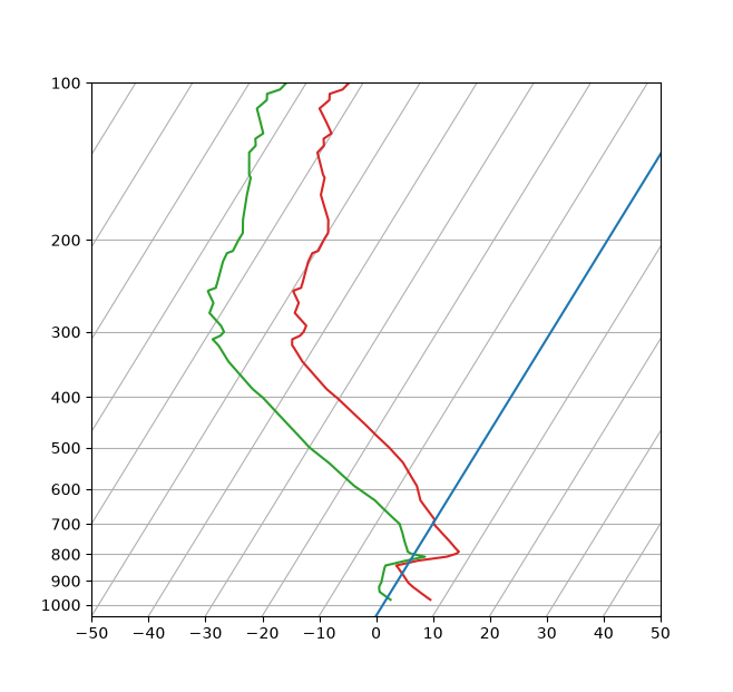
specialty_plots/topographic_hillshading
=======================
Source
"""
=======================
Topographic hillshading
=======================
Demonstrates the visual effect of varying blend mode and vertical exaggeration
on "hillshaded" plots.
Note that the "overlay" and "soft" blend modes work well for complex surfaces
such as this example, while the default "hsv" blend mode works best for smooth
surfaces such as many mathematical functions.
In most cases, hillshading is used purely for visual purposes, and *dx*/*dy*
can be safely ignored. In that case, you can tweak *vert_exag* (vertical
exaggeration) by trial and error to give the desired visual effect. However,
this example demonstrates how to use the *dx* and *dy* keyword arguments to
ensure that the *vert_exag* parameter is the true vertical exaggeration.
"""
import matplotlib.pyplot as plt
import numpy as np
from matplotlib.cbook import get_sample_data
from matplotlib.colors import LightSource
dem = get_sample_data('jacksboro_fault_dem.npz')
z = dem['elevation']
# -- Optional dx and dy for accurate vertical exaggeration --------------------
# If you need topographically accurate vertical exaggeration, or you don't want
# to guess at what *vert_exag* should be, you'll need to specify the cellsize
# of the grid (i.e. the *dx* and *dy* parameters). Otherwise, any *vert_exag*
# value you specify will be relative to the grid spacing of your input data
# (in other words, *dx* and *dy* default to 1.0, and *vert_exag* is calculated
# relative to those parameters). Similarly, *dx* and *dy* are assumed to be in
# the same units as your input z-values. Therefore, we'll need to convert the
# given dx and dy from decimal degrees to meters.
dx, dy = dem['dx'], dem['dy']
dy = 111200 * dy
dx = 111200 * dx * np.cos(np.radians(dem['ymin']))
# -----------------------------------------------------------------------------
# Shade from the northwest, with the sun 45 degrees from horizontal
ls = LightSource(azdeg=315, altdeg=45)
cmap = plt.colormaps["gist_earth"]
fig, axs = plt.subplots(nrows=4, ncols=3, figsize=(8, 9))
plt.setp(axs.flat, xticks=[], yticks=[])
# Vary vertical exaggeration and blend mode and plot all combinations
for col, ve in zip(axs.T, [0.1, 1, 10]):
# Show the hillshade intensity image in the first row
col[0].imshow(ls.hillshade(z, vert_exag=ve, dx=dx, dy=dy), cmap='gray')
# Place hillshaded plots with different blend modes in the rest of the rows
for ax, mode in zip(col[1:], ['hsv', 'overlay', 'soft']):
rgb = ls.shade(z, cmap=cmap, blend_mode=mode,
vert_exag=ve, dx=dx, dy=dy)
ax.imshow(rgb)
# Label rows and columns
for ax, ve in zip(axs[0], [0.1, 1, 10]):
ax.set_title(f'{ve}', size=18)
for ax, mode in zip(axs[:, 0], ['Hillshade', 'hsv', 'overlay', 'soft']):
ax.set_ylabel(mode, size=18)
# Group labels...
axs[0, 1].annotate('Vertical Exaggeration', (0.5, 1), xytext=(0, 30),
textcoords='offset points', xycoords='axes fraction',
ha='center', va='bottom', size=20)
axs[2, 0].annotate('Blend Mode', (0, 0.5), xytext=(-30, 0),
textcoords='offset points', xycoords='axes fraction',
ha='right', va='center', size=20, rotation=90)
fig.subplots_adjust(bottom=0.05, right=0.95)
plt.show()
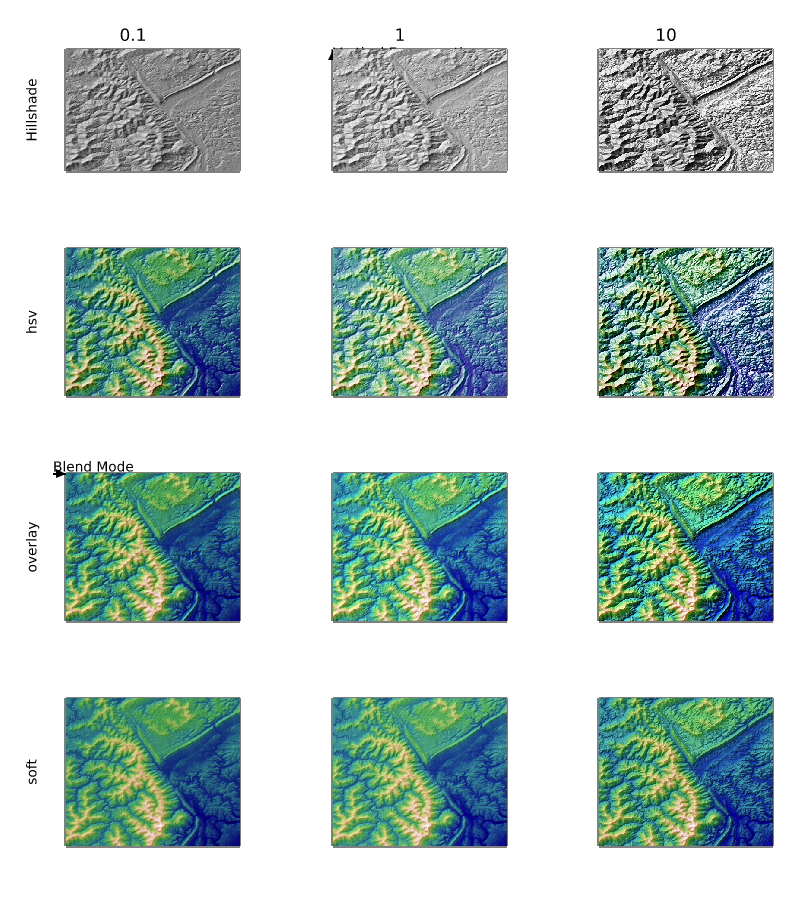
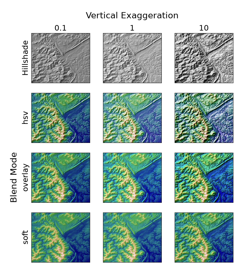
spines/centered_spines_with_arrows
===========================
Source
"""
===========================
Centered spines with arrows
===========================
This example shows a way to draw a "math textbook" style plot, where the
spines ("axes lines") are drawn at ``x = 0`` and ``y = 0``, and have arrows at
their ends.
"""
import matplotlib.pyplot as plt
import numpy as np
fig, ax = plt.subplots()
# Move the left and bottom spines to x = 0 and y = 0, respectively.
ax.spines[["left", "bottom"]].set_position(("data", 0))
# Hide the top and right spines.
ax.spines[["top", "right"]].set_visible(False)
# Draw arrows (as black triangles: ">k"/"^k") at the end of the axes. In each
# case, one of the coordinates (0) is a data coordinate (i.e., y = 0 or x = 0,
# respectively) and the other one (1) is an axes coordinate (i.e., at the very
# right/top of the axes). Also, disable clipping (clip_on=False) as the marker
# actually spills out of the Axes.
ax.plot(1, 0, ">k", transform=ax.get_yaxis_transform(), clip_on=False)
ax.plot(0, 1, "^k", transform=ax.get_xaxis_transform(), clip_on=False)
# Some sample data.
x = np.linspace(-0.5, 1., 100)
ax.plot(x, np.sin(x*np.pi))
plt.show()
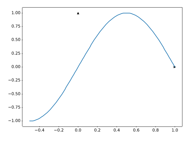
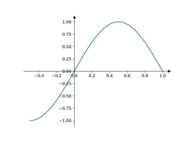
spines/spine_placement_demo
===============
Source
"""
===============
Spine placement
===============
The position of the axis spines can be influenced using `~.Spine.set_position`.
Note: If you want to obtain arrow heads at the ends of the axes, also check
out the :doc:`/gallery/spines/centered_spines_with_arrows` example.
"""
import matplotlib.pyplot as plt
import numpy as np
# %%
x = np.linspace(0, 2*np.pi, 100)
y = 2 * np.sin(x)
fig, ax_dict = plt.subplot_mosaic(
[['center', 'zero'],
['axes', 'data']]
)
fig.suptitle('Spine positions')
ax = ax_dict['center']
ax.set_title("'center'")
ax.plot(x, y)
ax.spines[['left', 'bottom']].set_position('center')
ax.spines[['top', 'right']].set_visible(False)
ax = ax_dict['zero']
ax.set_title("'zero'")
ax.plot(x, y)
ax.spines[['left', 'bottom']].set_position('zero')
ax.spines[['top', 'right']].set_visible(False)
ax = ax_dict['axes']
ax.set_title("'axes' (0.2, 0.2)")
ax.plot(x, y)
ax.spines.left.set_position(('axes', 0.2))
ax.spines.bottom.set_position(('axes', 0.2))
ax.spines[['top', 'right']].set_visible(False)
ax = ax_dict['data']
ax.set_title("'data' (1, 2)")
ax.plot(x, y)
ax.spines.left.set_position(('data', 1))
ax.spines.bottom.set_position(('data', 2))
ax.spines[['top', 'right']].set_visible(False)
plt.show()
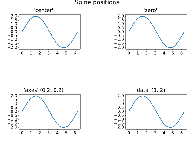
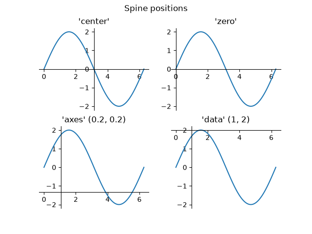
spines/spines
======
Source
"""
======
Spines
======
This demo compares:
- normal Axes, with spines on all four sides;
- an Axes with spines only on the left and bottom;
- an Axes using custom bounds to limit the extent of the spine.
Each `.axes.Axes` has a list of `.Spine` objects, accessible
via the container ``ax.spines``.
.. redirect-from:: /gallery/spines/spines_bounds
"""
import matplotlib.pyplot as plt
import numpy as np
x = np.linspace(0, 2 * np.pi, 100)
y = 2 * np.sin(x)
# Constrained layout makes sure the labels don't overlap the Axes.
fig, (ax0, ax1, ax2) = plt.subplots(nrows=3, layout='constrained')
ax0.plot(x, y)
ax0.set_title('normal spines')
ax1.plot(x, y)
ax1.set_title('bottom-left spines')
# Hide the right and top spines
ax1.spines.right.set_visible(False)
ax1.spines.top.set_visible(False)
ax2.plot(x, y)
ax2.set_title('spines with bounds limited to data range')
# Only draw spines for the data range, not in the margins
ax2.spines.bottom.set_bounds(x.min(), x.max())
ax2.spines.left.set_bounds(y.min(), y.max())
# Hide the right and top spines
ax2.spines.right.set_visible(False)
ax2.spines.top.set_visible(False)
plt.show()
# %%
#
# .. admonition:: References
#
# The use of the following functions, methods, classes and modules is shown
# in this example:
#
# - `matplotlib.artist.Artist.set_visible`
# - `matplotlib.spines.Spine.set_bounds`
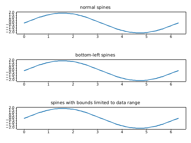
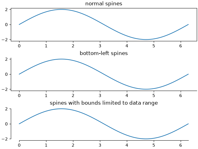
spines/spines_dropped
==============
Source
"""
==============
Dropped spines
==============
Demo of spines offset from the axes (a.k.a. "dropped spines").
"""
import matplotlib.pyplot as plt
import numpy as np
def adjust_spines(ax, visible_spines):
ax.label_outer(remove_inner_ticks=True)
ax.grid(color='0.9')
for loc, spine in ax.spines.items():
if loc in visible_spines:
spine.set_position(('outward', 10)) # outward by 10 points
else:
spine.set_visible(False)
x = np.linspace(0, 2 * np.pi, 100)
fig, axs = plt.subplots(2, 2)
axs[0, 0].plot(x, np.sin(x))
axs[0, 1].plot(x, np.cos(x))
axs[1, 0].plot(x, -np.cos(x))
axs[1, 1].plot(x, -np.sin(x))
adjust_spines(axs[0, 0], ['left'])
adjust_spines(axs[0, 1], [])
adjust_spines(axs[1, 0], ['left', 'bottom'])
adjust_spines(axs[1, 1], ['bottom'])
plt.show()
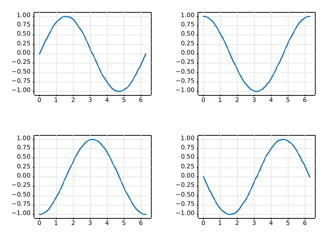
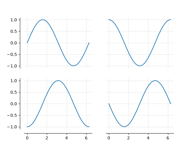
statistics/boxplot
=================================
Source
"""
=================================
Artist customization in box plots
=================================
This example demonstrates how to use the various keyword arguments to fully
customize box plots. The first figure demonstrates how to remove and add
individual components (note that the mean is the only value not shown by
default). The second figure demonstrates how the styles of the artists can be
customized. It also demonstrates how to set the limit of the whiskers to
specific percentiles (lower right Axes)
A good general reference on boxplots and their history can be found here:
https://vita.had.co.nz/papers/boxplots.pdf
"""
import matplotlib.pyplot as plt
import numpy as np
# fake data
np.random.seed(19680801)
data = np.random.lognormal(size=(37, 4), mean=1.5, sigma=1.75)
labels = list('ABCD')
fs = 10 # fontsize
# %%
# Demonstrate how to toggle the display of different elements:
fig, axs = plt.subplots(nrows=2, ncols=3, figsize=(6, 6), sharey=True)
axs[0, 0].boxplot(data, tick_labels=labels)
axs[0, 0].set_title('Default', fontsize=fs)
axs[0, 1].boxplot(data, tick_labels=labels, showmeans=True)
axs[0, 1].set_title('showmeans=True', fontsize=fs)
axs[0, 2].boxplot(data, tick_labels=labels, showmeans=True, meanline=True)
axs[0, 2].set_title('showmeans=True,\nmeanline=True', fontsize=fs)
axs[1, 0].boxplot(data, tick_labels=labels, showbox=False, showcaps=False)
tufte_title = 'Tufte Style \n(showbox=False,\nshowcaps=False)'
axs[1, 0].set_title(tufte_title, fontsize=fs)
axs[1, 1].boxplot(data, tick_labels=labels, notch=True, bootstrap=10000)
axs[1, 1].set_title('notch=True,\nbootstrap=10000', fontsize=fs)
axs[1, 2].boxplot(data, tick_labels=labels, showfliers=False)
axs[1, 2].set_title('showfliers=False', fontsize=fs)
for ax in axs.flat:
ax.set_yscale('log')
ax.set_yticklabels([])
fig.subplots_adjust(hspace=0.4)
plt.show()
# %%
# Demonstrate how to customize the display different elements:
boxprops = dict(linestyle='--', linewidth=3, color='darkgoldenrod')
flierprops = dict(marker='o', markerfacecolor='green', markersize=12,
markeredgecolor='none')
medianprops = dict(linestyle='-.', linewidth=2.5, color='firebrick')
meanpointprops = dict(marker='D', markeredgecolor='black',
markerfacecolor='firebrick')
meanlineprops = dict(linestyle='--', linewidth=2.5, color='purple')
fig, axs = plt.subplots(nrows=2, ncols=3, figsize=(6, 6), sharey=True)
axs[0, 0].boxplot(data, boxprops=boxprops)
axs[0, 0].set_title('Custom boxprops', fontsize=fs)
axs[0, 1].boxplot(data, flierprops=flierprops, medianprops=medianprops)
axs[0, 1].set_title('Custom medianprops\nand flierprops', fontsize=fs)
axs[0, 2].boxplot(data, whis=(0, 100))
axs[0, 2].set_title('whis=(0, 100)', fontsize=fs)
axs[1, 0].boxplot(data, meanprops=meanpointprops, meanline=False,
showmeans=True)
axs[1, 0].set_title('Custom mean\nas point', fontsize=fs)
axs[1, 1].boxplot(data, meanprops=meanlineprops, meanline=True,
showmeans=True)
axs[1, 1].set_title('Custom mean\nas line', fontsize=fs)
axs[1, 2].boxplot(data, whis=[15, 85])
axs[1, 2].set_title('whis=[15, 85]\n#percentiles', fontsize=fs)
for ax in axs.flat:
ax.set_yscale('log')
ax.set_yticklabels([])
fig.suptitle("I never said they'd be pretty")
fig.subplots_adjust(hspace=0.4)
plt.show()
# %%
#
# .. tags:: plot-type: boxplot, domain: statistics
#
# .. admonition:: References
#
# The use of the following functions, methods, classes and modules is shown
# in this example:
#
# - `matplotlib.axes.Axes.boxplot` / `matplotlib.pyplot.boxplot`
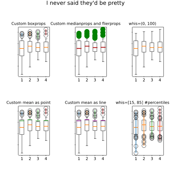
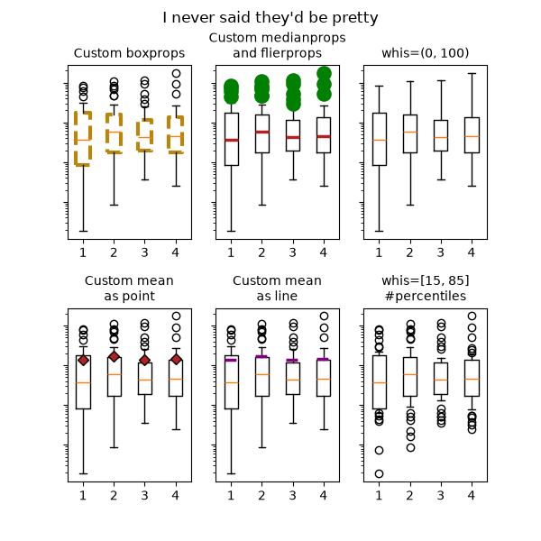
statistics/boxplot_color
=================================
Source
"""
=================================
Box plots with custom fill colors
=================================
To color each box of a box plot individually:
1) use the keyword argument ``patch_artist=True`` to create filled boxes.
2) loop through the created boxes and adapt their color.
"""
import matplotlib.pyplot as plt
import numpy as np
np.random.seed(19680801)
fruit_weights = [
np.random.normal(130, 10, size=100),
np.random.normal(125, 20, size=100),
np.random.normal(120, 30, size=100),
]
labels = ['peaches', 'oranges', 'tomatoes']
colors = ['peachpuff', 'orange', 'tomato']
fig, ax = plt.subplots()
ax.set_ylabel('fruit weight (g)')
bplot = ax.boxplot(fruit_weights,
patch_artist=True, # fill with color
tick_labels=labels) # will be used to label x-ticks
# fill with colors
for patch, color in zip(bplot['boxes'], colors):
patch.set_facecolor(color)
plt.show()
# %%
#
# .. tags:: styling: color, domain: statistics, plot-type: boxplot
#
# .. admonition:: References
#
# The use of the following functions, methods, classes and modules is shown
# in this example:
#
# - `matplotlib.axes.Axes.boxplot` / `matplotlib.pyplot.boxplot`
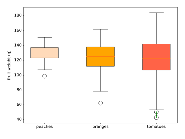
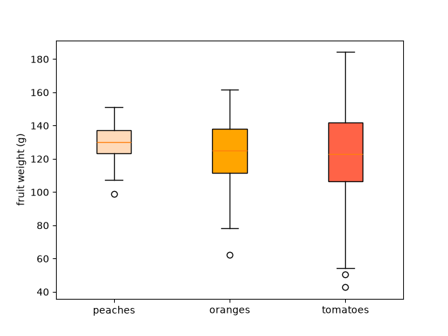
statistics/boxplot_demo
========
Source
"""
========
Boxplots
========
Visualizing boxplots with matplotlib.
The following examples show off how to visualize boxplots with
Matplotlib. There are many options to control their appearance and
the statistics that they use to summarize the data.
.. redirect-from:: /gallery/pyplots/boxplot_demo_pyplot
"""
import matplotlib.pyplot as plt
import numpy as np
from matplotlib.patches import Polygon
# Fixing random state for reproducibility
np.random.seed(19680801)
# fake up some data
spread = np.random.rand(50) * 100
center = np.ones(25) * 50
flier_high = np.random.rand(10) * 100 + 100
flier_low = np.random.rand(10) * -100
data = np.concatenate((spread, center, flier_high, flier_low))
fig, axs = plt.subplots(2, 3)
# basic plot
axs[0, 0].boxplot(data)
axs[0, 0].set_title('basic plot')
# notched plot
axs[0, 1].boxplot(data, notch=True)
axs[0, 1].set_title('notched plot')
# change outlier point symbols
axs[0, 2].boxplot(data, sym='gD')
axs[0, 2].set_title('change outlier\npoint symbols')
# don't show outlier points
axs[1, 0].boxplot(data, sym='')
axs[1, 0].set_title("don't show\noutlier points")
# horizontal boxes
axs[1, 1].boxplot(data, sym='rs', orientation='horizontal')
axs[1, 1].set_title('horizontal boxes')
# change whisker length
axs[1, 2].boxplot(data, sym='rs', orientation='horizontal', whis=0.75)
axs[1, 2].set_title('change whisker length')
fig.subplots_adjust(left=0.08, right=0.98, bottom=0.05, top=0.9,
hspace=0.4, wspace=0.3)
# fake up some more data
spread = np.random.rand(50) * 100
center = np.ones(25) * 40
flier_high = np.random.rand(10) * 100 + 100
flier_low = np.random.rand(10) * -100
d2 = np.concatenate((spread, center, flier_high, flier_low))
# Making a 2-D array only works if all the columns are the
# same length. If they are not, then use a list instead.
# This is actually more efficient because boxplot converts
# a 2-D array into a list of vectors internally anyway.
data = [data, d2, d2[::2]]
# Multiple box plots on one Axes
fig, ax = plt.subplots()
ax.boxplot(data)
plt.show()
# %%
# Below we'll generate data from five different probability distributions,
# each with different characteristics. We want to play with how an IID
# bootstrap resample of the data preserves the distributional
# properties of the original sample, and a boxplot is one visual tool
# to make this assessment
random_dists = ['Normal(1, 1)', 'Lognormal(1, 1)', 'Exp(1)', 'Gumbel(6, 4)',
'Triangular(2, 9, 11)']
N = 500
norm = np.random.normal(1, 1, N)
logn = np.random.lognormal(1, 1, N)
expo = np.random.exponential(1, N)
gumb = np.random.gumbel(6, 4, N)
tria = np.random.triangular(2, 9, 11, N)
# Generate some random indices that we'll use to resample the original data
# arrays. For code brevity, just use the same random indices for each array
bootstrap_indices = np.random.randint(0, N, N)
data = [
norm, norm[bootstrap_indices],
logn, logn[bootstrap_indices],
expo, expo[bootstrap_indices],
gumb, gumb[bootstrap_indices],
tria, tria[bootstrap_indices],
]
fig, ax1 = plt.subplots(figsize=(10, 6))
fig.canvas.manager.set_window_title('A Boxplot Example')
fig.subplots_adjust(left=0.075, right=0.95, top=0.9, bottom=0.25)
bp = ax1.boxplot(data, notch=False, sym='+', orientation='vertical', whis=1.5)
plt.setp(bp['boxes'], color='black')
plt.setp(bp['whiskers'], color='black')
plt.setp(bp['fliers'], color='red', marker='+')
# Add a horizontal grid to the plot, but make it very light in color
# so we can use it for reading data values but not be distracting
ax1.yaxis.grid(True, linestyle='-', which='major', color='lightgrey',
alpha=0.5)
ax1.set(
axisbelow=True, # Hide the grid behind plot objects
title='Comparison of IID Bootstrap Resampling Across Five Distributions',
xlabel='Distribution',
ylabel='Value',
)
# Now fill the boxes with desired colors
box_colors = ['darkkhaki', 'royalblue']
num_boxes = len(data)
medians = np.empty(num_boxes)
for i in range(num_boxes):
box = bp['boxes'][i]
box_x = []
box_y = []
for j in range(5):
box_x.append(box.get_xdata()[j])
box_y.append(box.get_ydata()[j])
box_coords = np.column_stack([box_x, box_y])
# Alternate between Dark Khaki and Royal Blue
ax1.add_patch(Polygon(box_coords, facecolor=box_colors[i % 2]))
# Now draw the median lines back over what we just filled in
med = bp['medians'][i]
median_x = []
median_y = []
for j in range(2):
median_x.append(med.get_xdata()[j])
median_y.append(med.get_ydata()[j])
ax1.plot(median_x, median_y, 'k')
medians[i] = median_y[0]
# Finally, overplot the sample averages, with horizontal alignment
# in the center of each box
ax1.plot(np.average(med.get_xdata()), np.average(data[i]),
color='w', marker='*', markeredgecolor='k')
# Set the axes ranges and axes labels
ax1.set_xlim(0.5, num_boxes + 0.5)
top = 40
bottom = -5
ax1.set_ylim(bottom, top)
ax1.set_xticklabels(np.repeat(random_dists, 2),
rotation=45, fontsize=8)
# Due to the Y-axis scale being different across samples, it can be
# hard to compare differences in medians across the samples. Add upper
# X-axis tick labels with the sample medians to aid in comparison
# (just use two decimal places of precision)
pos = np.arange(num_boxes) + 1
upper_labels = [str(round(s, 2)) for s in medians]
weights = ['bold', 'semibold']
for tick, label in zip(range(num_boxes), ax1.get_xticklabels()):
k = tick % 2
ax1.text(pos[tick], .95, upper_labels[tick],
transform=ax1.get_xaxis_transform(),
horizontalalignment='center', size='x-small',
weight=weights[k], color=box_colors[k])
# Finally, add a basic legend
fig.text(0.80, 0.08, f'{N} Random Numbers',
backgroundcolor=box_colors[0], color='black', weight='roman',
size='x-small')
fig.text(0.80, 0.045, 'IID Bootstrap Resample',
backgroundcolor=box_colors[1],
color='white', weight='roman', size='x-small')
fig.text(0.80, 0.015, '*', color='white', backgroundcolor='silver',
weight='roman', size='medium')
fig.text(0.815, 0.013, ' Average Value', color='black', weight='roman',
size='x-small')
plt.show()
# %%
# Here we write a custom function to bootstrap confidence intervals.
# We can then use the boxplot along with this function to show these intervals.
def fake_bootstrapper(n):
"""
This is just a placeholder for the user's method of
bootstrapping the median and its confidence intervals.
Returns an arbitrary median and confidence interval packed into a tuple.
"""
if n == 1:
med = 0.1
ci = (-0.25, 0.25)
else:
med = 0.2
ci = (-0.35, 0.50)
return med, ci
inc = 0.1
e1 = np.random.normal(0, 1, size=500)
e2 = np.random.normal(0, 1, size=500)
e3 = np.random.normal(0, 1 + inc, size=500)
e4 = np.random.normal(0, 1 + 2*inc, size=500)
treatments = [e1, e2, e3, e4]
med1, ci1 = fake_bootstrapper(1)
med2, ci2 = fake_bootstrapper(2)
medians = [None, None, med1, med2]
conf_intervals = [None, None, ci1, ci2]
fig, ax = plt.subplots()
pos = np.arange(len(treatments)) + 1
bp = ax.boxplot(treatments, sym='k+', positions=pos,
notch=True, bootstrap=5000,
usermedians=medians,
conf_intervals=conf_intervals)
ax.set_xlabel('treatment')
ax.set_ylabel('response')
plt.setp(bp['whiskers'], color='k', linestyle='-')
plt.setp(bp['fliers'], markersize=3.0)
plt.show()
# %%
# Here we customize the widths of the caps .
x = np.linspace(-7, 7, 140)
x = np.hstack([-25, x, 25])
fig, ax = plt.subplots()
ax.boxplot([x, x], notch=True, capwidths=[0.01, 0.2])
plt.show()
# %%
#
# .. tags:: domain: statistics, plot-type: boxplot
#
# .. admonition:: References
#
# The use of the following functions, methods, classes and modules is shown
# in this example:
#
# - `matplotlib.axes.Axes.boxplot` / `matplotlib.pyplot.boxplot`
# - `matplotlib.artist.Artist.set` / `matplotlib.pyplot.setp`
AttributeError: NoneType has no set_color
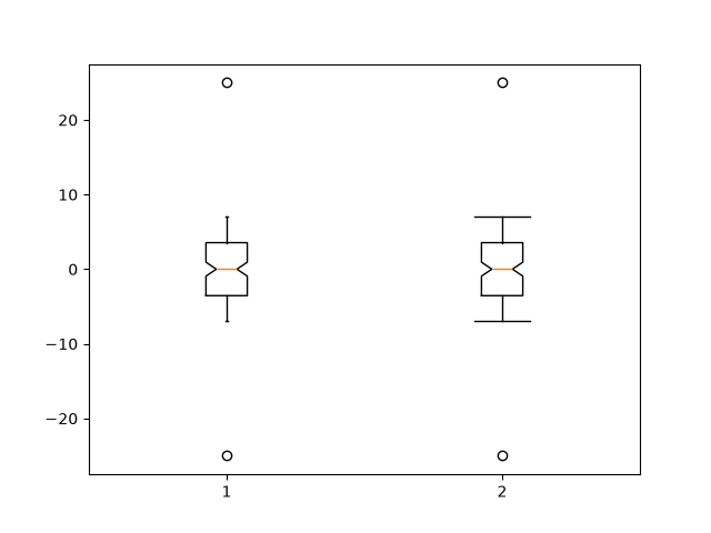
statistics/boxplot_vs_violin
===================================
Source
"""
===================================
Box plot vs. violin plot comparison
===================================
Note that although violin plots are closely related to Tukey's (1977)
box plots, they add useful information such as the distribution of the
sample data (density trace).
By default, box plots show data points outside 1.5 * the inter-quartile
range as outliers above or below the whiskers whereas violin plots show
the whole range of the data.
A good general reference on boxplots and their history can be found
here: https://vita.had.co.nz/papers/boxplots.pdf
Violin plots require matplotlib >= 1.4.
Violin plots show the distribution of the data as a rotated kernel density
estimate (KDE) along with summary statistics similar to a box plot.
For more information on violin plots, see:
https://en.wikipedia.org/wiki/Violin_plot
"""
import matplotlib.pyplot as plt
import numpy as np
fig, axs = plt.subplots(nrows=1, ncols=2, figsize=(9, 4))
# Fixing random state for reproducibility
np.random.seed(19680801)
# generate some random test data
all_data = [np.random.normal(0, std, 100) for std in range(6, 10)]
# plot violin plot
axs[0].violinplot(all_data,
showmeans=False,
showmedians=True)
axs[0].set_title('Violin plot')
# plot box plot
axs[1].boxplot(all_data)
axs[1].set_title('Box plot')
# adding horizontal grid lines
for ax in axs:
ax.yaxis.grid(True)
ax.set_xticks([y + 1 for y in range(len(all_data))],
labels=['x1', 'x2', 'x3', 'x4'])
ax.set_xlabel('Four separate samples')
ax.set_ylabel('Observed values')
plt.show()
# %%
#
# .. tags:: plot-type: violin, plot-type: boxplot, domain: statistics
#
# .. admonition:: References
#
# The use of the following functions, methods, classes and modules is shown
# in this example:
#
# - `matplotlib.axes.Axes.boxplot` / `matplotlib.pyplot.boxplot`
# - `matplotlib.axes.Axes.violinplot` / `matplotlib.pyplot.violinplot`
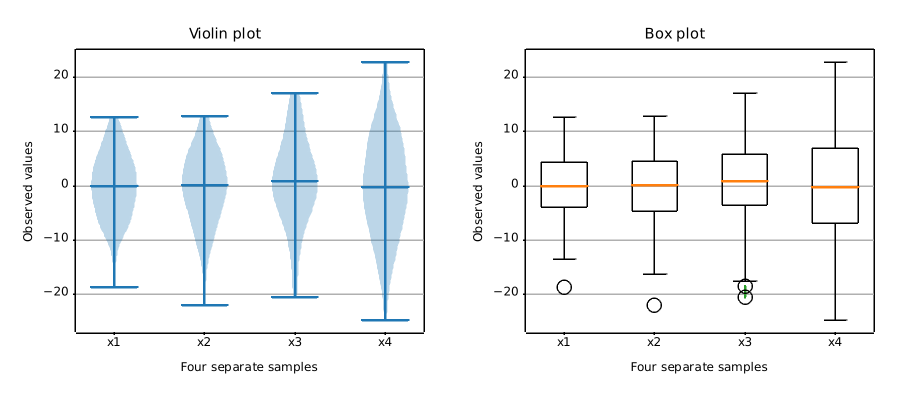
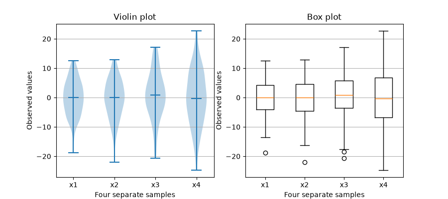
statistics/bxp
=============================================
Source
"""
=============================================
Separate calculation and plotting of boxplots
=============================================
Drawing a `~.axes.Axes.boxplot` for a given data set, consists of two main operations,
that can also be used separately:
1. Calculating the boxplot statistics: `matplotlib.cbook.boxplot_stats`
2. Drawing the boxplot: `matplotlib.axes.Axes.bxp`
Thus, ``ax.boxplot(data)`` is equivalent to ::
stats = cbook.boxplot_stats(data)
ax.bxp(stats)
All styling keyword arguments are identical between `~.axes.Axes.boxplot` and
`~.axes.Axes.bxp`, and they are passed through from `~.axes.Axes.boxplot` to
`~.axes.Axes.bxp`. However, the *tick_labels* parameter of `~.axes.Axes.boxplot`
translates to a generic *labels* parameter in `.boxplot_stats`, because the labels are
data-related and attached to the returned per-dataset dictionaries.
The following code demonstrates the equivalence between the two methods.
"""
# sphinx_gallery_thumbnail_number = 2
import matplotlib.pyplot as plt
import numpy as np
from matplotlib import cbook
np.random.seed(19680801)
data = np.random.randn(20, 3)
fig, (ax1, ax2) = plt.subplots(1, 2)
# single boxplot call
ax1.boxplot(data, tick_labels=['A', 'B', 'C'],
patch_artist=True, boxprops={'facecolor': 'bisque'})
# separate calculation of statistics and plotting
stats = cbook.boxplot_stats(data, labels=['A', 'B', 'C'])
ax2.bxp(stats, patch_artist=True, boxprops={'facecolor': 'bisque'})
# %%
# Using the separate functions allows to pre-calculate statistics, in case you need
# them explicitly for other purposes, or to reuse the statistics for multiple plots.
#
# Conversely, you can also use the `~.axes.Axes.bxp` function directly, if you already
# have the statistical parameters:
fig, ax = plt.subplots()
stats = [
dict(med=0, q1=-1, q3=1, whislo=-2, whishi=2, fliers=[-4, -3, 3, 4], label='A'),
dict(med=0, q1=-2, q3=2, whislo=-3, whishi=3, fliers=[], label='B'),
dict(med=0, q1=-3, q3=3, whislo=-4, whishi=4, fliers=[], label='C'),
]
ax.bxp(stats, patch_artist=True, boxprops={'facecolor': 'bisque'})
plt.show()
# %%
#
# .. tags:: plot-type: specialty, domain: statistics
#
# .. admonition:: References
#
# The use of the following functions, methods, classes and modules is shown
# in this example:
#
# - `matplotlib.axes.Axes.bxp`
# - `matplotlib.axes.Axes.boxplot`
# - `matplotlib.cbook.boxplot_stats`
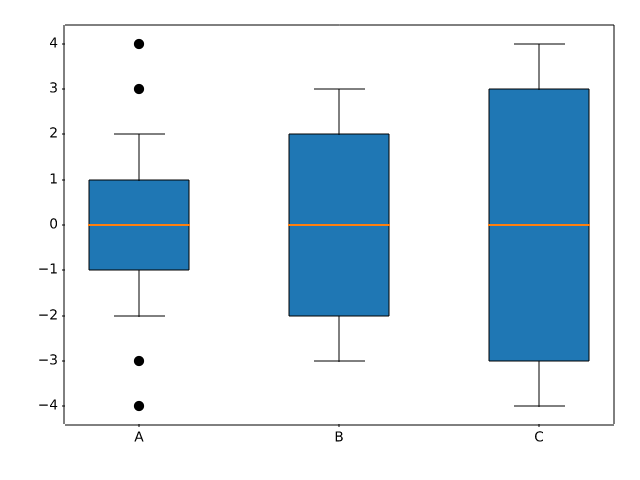
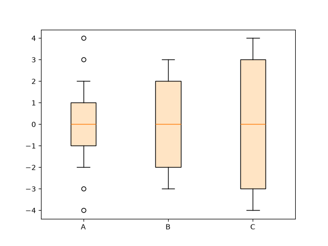
statistics/cohere
=====================================
Source
"""
=====================================
Plotting the coherence of two signals
=====================================
An example showing how to plot the coherence of two signals using `~.Axes.cohere`.
.. redirect-from:: /gallery/lines_bars_and_markers/cohere
"""
import matplotlib.pyplot as plt
import numpy as np
# Fixing random state for reproducibility
np.random.seed(19680801)
dt = 0.01
t = np.arange(0, 30, dt)
nse1 = np.random.randn(len(t)) # white noise 1
nse2 = np.random.randn(len(t)) # white noise 2
# Two signals with a coherent part at 10 Hz and a random part
s1 = np.sin(2 * np.pi * 10 * t) + nse1
s2 = np.sin(2 * np.pi * 10 * t) + nse2
fig, axs = plt.subplots(2, 1, layout='constrained')
axs[0].plot(t, s1, t, s2)
axs[0].set_xlim(0, 2)
axs[0].set_xlabel('Time (s)')
axs[0].set_ylabel('s1 and s2')
axs[0].grid(True)
cxy, f = axs[1].cohere(s1, s2, NFFT=256, Fs=1. / dt)
axs[1].set_ylabel('Coherence')
plt.show()
# %%
# .. tags::
#
# domain: signal-processing
# plot-type: line
# level: beginner
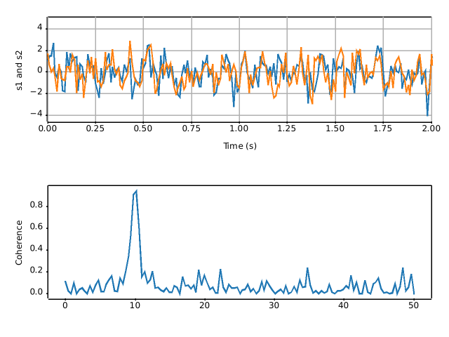
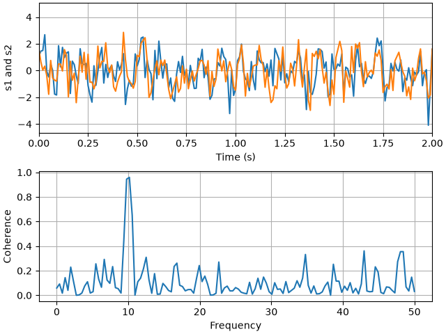
statistics/confidence_ellipse
======================================================
Source
"""
======================================================
Plot a confidence ellipse of a two-dimensional dataset
======================================================
This example shows how to plot a confidence ellipse of a
two-dimensional dataset, using its pearson correlation coefficient.
The approach that is used to obtain the correct geometry is
explained and proved here:
https://carstenschelp.github.io/2018/09/14/Plot_Confidence_Ellipse_001.html
The method avoids the use of an iterative eigen decomposition algorithm
and makes use of the fact that a normalized covariance matrix (composed of
pearson correlation coefficients and ones) is particularly easy to handle.
"""
import matplotlib.pyplot as plt
import numpy as np
from matplotlib.patches import Ellipse
import matplotlib.transforms as transforms
# %%
#
# The plotting function itself
# """"""""""""""""""""""""""""
#
# This function plots the confidence ellipse of the covariance of the given
# array-like variables x and y. The ellipse is plotted into the given
# Axes object *ax*.
#
# The radiuses of the ellipse can be controlled by n_std which is the number
# of standard deviations. The default value is 3 which makes the ellipse
# enclose 98.9% of the points if the data is normally distributed
# like in these examples (3 standard deviations in 1-D contain 99.7%
# of the data, which is 98.9% of the data in 2-D).
def confidence_ellipse(x, y, ax, n_std=3.0, facecolor='none', **kwargs):
"""
Create a plot of the covariance confidence ellipse of *x* and *y*.
Parameters
----------
x, y : array-like, shape (n, )
Input data.
ax : matplotlib.axes.Axes
The Axes object to draw the ellipse into.
n_std : float
The number of standard deviations to determine the ellipse's radiuses.
**kwargs
Forwarded to `~matplotlib.patches.Ellipse`
Returns
-------
matplotlib.patches.Ellipse
"""
if x.size != y.size:
raise ValueError("x and y must be the same size")
cov = np.cov(x, y)
pearson = cov[0, 1]/np.sqrt(cov[0, 0] * cov[1, 1])
# Using a special case to obtain the eigenvalues of this
# two-dimensional dataset.
ell_radius_x = np.sqrt(1 + pearson)
ell_radius_y = np.sqrt(1 - pearson)
ellipse = Ellipse((0, 0), width=ell_radius_x * 2, height=ell_radius_y * 2,
facecolor=facecolor, **kwargs)
# Calculating the standard deviation of x from
# the squareroot of the variance and multiplying
# with the given number of standard deviations.
scale_x = np.sqrt(cov[0, 0]) * n_std
mean_x = np.mean(x)
# calculating the standard deviation of y ...
scale_y = np.sqrt(cov[1, 1]) * n_std
mean_y = np.mean(y)
transf = transforms.Affine2D() \
.rotate_deg(45) \
.scale(scale_x, scale_y) \
.translate(mean_x, mean_y)
ellipse.set_transform(transf + ax.transData)
return ax.add_patch(ellipse)
# %%
#
# A helper function to create a correlated dataset
# """"""""""""""""""""""""""""""""""""""""""""""""
#
# Creates a random two-dimensional dataset with the specified
# two-dimensional mean (mu) and dimensions (scale).
# The correlation can be controlled by the param 'dependency',
# a 2x2 matrix.
def get_correlated_dataset(n, dependency, mu, scale):
latent = np.random.randn(n, 2)
dependent = latent.dot(dependency)
scaled = dependent * scale
scaled_with_offset = scaled + mu
# return x and y of the new, correlated dataset
return scaled_with_offset[:, 0], scaled_with_offset[:, 1]
# %%
#
# Positive, negative and weak correlation
# """""""""""""""""""""""""""""""""""""""
#
# Note that the shape for the weak correlation (right) is an ellipse,
# not a circle because x and y are differently scaled.
# However, the fact that x and y are uncorrelated is shown by
# the axes of the ellipse being aligned with the x- and y-axis
# of the coordinate system.
np.random.seed(0)
PARAMETERS = {
'Positive correlation': [[0.85, 0.35],
[0.15, -0.65]],
'Negative correlation': [[0.9, -0.4],
[0.1, -0.6]],
'Weak correlation': [[1, 0],
[0, 1]],
}
mu = 2, 4
scale = 3, 5
fig, axs = plt.subplots(1, 3, figsize=(9, 3))
for ax, (title, dependency) in zip(axs, PARAMETERS.items()):
x, y = get_correlated_dataset(800, dependency, mu, scale)
ax.scatter(x, y, s=0.5)
ax.axvline(c='grey', lw=1)
ax.axhline(c='grey', lw=1)
confidence_ellipse(x, y, ax, edgecolor='red')
ax.scatter(mu[0], mu[1], c='red', s=3)
ax.set_title(title)
plt.show()
# %%
#
# Different number of standard deviations
# """""""""""""""""""""""""""""""""""""""
#
# A plot with n_std = 3 (blue), 2 (purple) and 1 (red)
fig, ax_nstd = plt.subplots(figsize=(6, 6))
dependency_nstd = [[0.8, 0.75],
[-0.2, 0.35]]
mu = 0, 0
scale = 8, 5
ax_nstd.axvline(c='grey', lw=1)
ax_nstd.axhline(c='grey', lw=1)
x, y = get_correlated_dataset(500, dependency_nstd, mu, scale)
ax_nstd.scatter(x, y, s=0.5)
confidence_ellipse(x, y, ax_nstd, n_std=1,
label=r'$1\sigma$', edgecolor='firebrick')
confidence_ellipse(x, y, ax_nstd, n_std=2,
label=r'$2\sigma$', edgecolor='fuchsia', linestyle='--')
confidence_ellipse(x, y, ax_nstd, n_std=3,
label=r'$3\sigma$', edgecolor='blue', linestyle=':')
ax_nstd.scatter(mu[0], mu[1], c='red', s=3)
ax_nstd.set_title('Different standard deviations')
ax_nstd.legend()
plt.show()
# %%
#
# Using the keyword arguments
# """""""""""""""""""""""""""
#
# Use the keyword arguments specified for `matplotlib.patches.Patch` in order
# to have the ellipse rendered in different ways.
fig, ax_kwargs = plt.subplots(figsize=(6, 6))
dependency_kwargs = [[-0.8, 0.5],
[-0.2, 0.5]]
mu = 2, -3
scale = 6, 5
ax_kwargs.axvline(c='grey', lw=1)
ax_kwargs.axhline(c='grey', lw=1)
x, y = get_correlated_dataset(500, dependency_kwargs, mu, scale)
# Plot the ellipse with zorder=0 in order to demonstrate
# its transparency (caused by the use of alpha).
confidence_ellipse(x, y, ax_kwargs,
alpha=0.5, facecolor='pink', edgecolor='purple', zorder=0)
ax_kwargs.scatter(x, y, s=0.5)
ax_kwargs.scatter(mu[0], mu[1], c='red', s=3)
ax_kwargs.set_title('Using keyword arguments')
fig.subplots_adjust(hspace=0.25)
plt.show()
# %%
#
# .. tags::
#
# plot-type: specialty
# plot-type: scatter
# component: ellipse
# component: patch
# domain: statistics
#
# .. admonition:: References
#
# The use of the following functions, methods, classes and modules is shown
# in this example:
#
# - `matplotlib.transforms.Affine2D`
# - `matplotlib.patches.Ellipse`
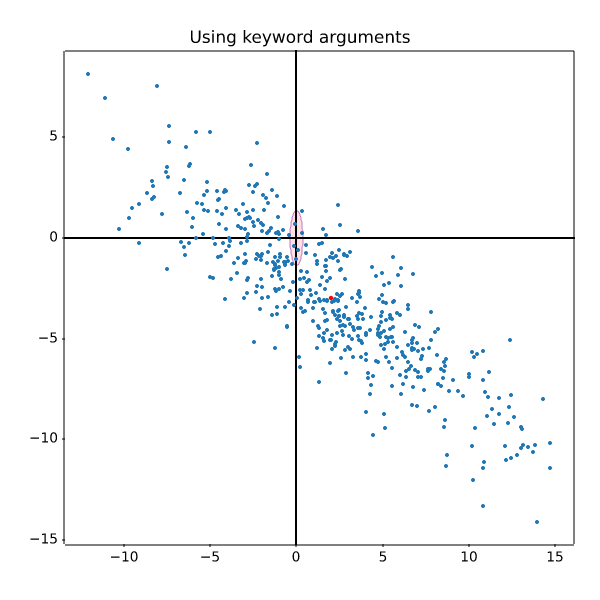
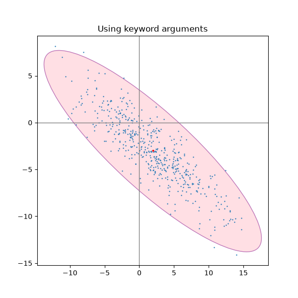
statistics/csd_demo
============================
Source
"""
============================
Cross spectral density (CSD)
============================
Plot the cross spectral density (CSD) of two signals using `~.Axes.csd`.
.. redirect-from:: /gallery/lines_bars_and_markers/csd_demo
"""
import matplotlib.pyplot as plt
import numpy as np
fig, (ax1, ax2) = plt.subplots(2, 1, layout='constrained')
dt = 0.01
t = np.arange(0, 30, dt)
# Fixing random state for reproducibility
np.random.seed(19680801)
nse1 = np.random.randn(len(t)) # white noise 1
nse2 = np.random.randn(len(t)) # white noise 2
r = np.exp(-t / 0.05)
cnse1 = np.convolve(nse1, r, mode='same') * dt # colored noise 1
cnse2 = np.convolve(nse2, r, mode='same') * dt # colored noise 2
# two signals with a coherent part and a random part
s1 = 0.01 * np.sin(2 * np.pi * 10 * t) + cnse1
s2 = 0.01 * np.sin(2 * np.pi * 10 * t) + cnse2
ax1.plot(t, s1, t, s2)
ax1.set_xlim(0, 5)
ax1.set_xlabel('Time (s)')
ax1.set_ylabel('s1 and s2')
ax1.grid(True)
cxy, f = ax2.csd(s1, s2, NFFT=256, Fs=1. / dt)
ax2.set_ylabel('CSD (dB)')
plt.show()
# %%
# .. tags::
#
# domain: signal-processing
# plot-type: line
# level: beginner
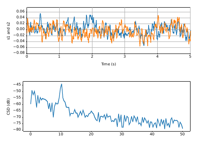
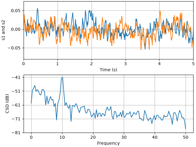
statistics/curve_error_band
=====================
Source
"""
=====================
Curve with error band
=====================
This example illustrates how to draw an error band around a parametrized curve.
A parametrized curve x(t), y(t) can directly be drawn using `~.Axes.plot`.
.. redirect-from:: /gallery/lines_bars_and_markers/curve_error_band
"""
# sphinx_gallery_thumbnail_number = 2
import matplotlib.pyplot as plt
import numpy as np
from matplotlib.patches import PathPatch
from matplotlib.path import Path
N = 400
t = np.linspace(0, 2 * np.pi, N)
r = 0.5 + np.cos(t)
x, y = r * np.cos(t), r * np.sin(t)
fig, ax = plt.subplots()
ax.plot(x, y, "k")
ax.set(aspect=1)
# %%
# An error band can be used to indicate the uncertainty of the curve.
# In this example we assume that the error can be given as a scalar *err*
# that describes the uncertainty perpendicular to the curve in every point.
#
# We visualize this error as a colored band around the path using a
# `.PathPatch`. The patch is created from two path segments *(xp, yp)*, and
# *(xn, yn)* that are shifted by +/- *err* perpendicular to the curve *(x, y)*.
#
# Note: This method of using a `.PathPatch` is suited to arbitrary curves in
# 2D. If you just have a standard y-vs.-x plot, you can use the simpler
# `~.Axes.fill_between` method (see also
# :doc:`/gallery/lines_bars_and_markers/fill_between_demo`).
def draw_error_band(ax, x, y, err, **kwargs):
# Calculate normals via centered finite differences (except the first point
# which uses a forward difference and the last point which uses a backward
# difference).
dx = np.concatenate([[x[1] - x[0]], x[2:] - x[:-2], [x[-1] - x[-2]]])
dy = np.concatenate([[y[1] - y[0]], y[2:] - y[:-2], [y[-1] - y[-2]]])
l = np.hypot(dx, dy)
nx = dy / l
ny = -dx / l
# end points of errors
xp = x + nx * err
yp = y + ny * err
xn = x - nx * err
yn = y - ny * err
vertices = np.block([[xp, xn[::-1]],
[yp, yn[::-1]]]).T
codes = np.full(len(vertices), Path.LINETO)
codes[0] = codes[len(xp)] = Path.MOVETO
path = Path(vertices, codes)
ax.add_patch(PathPatch(path, **kwargs))
_, axs = plt.subplots(1, 2, layout='constrained', sharex=True, sharey=True)
errs = [
(axs[0], "constant error", 0.05),
(axs[1], "variable error", 0.05 * np.sin(2 * t) ** 2 + 0.04),
]
for i, (ax, title, err) in enumerate(errs):
ax.set(title=title, aspect=1, xticks=[], yticks=[])
ax.plot(x, y, "k")
draw_error_band(ax, x, y, err=err,
facecolor=f"C{i}", edgecolor="none", alpha=.3)
plt.show()
# %%
#
# .. admonition:: References
#
# The use of the following functions, methods, classes and modules is shown
# in this example:
#
# - `matplotlib.patches.PathPatch`
# - `matplotlib.path.Path`
#
# .. tags::
#
# component: error
# plot-type: line
# level: intermediate
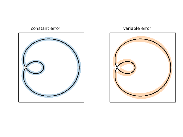
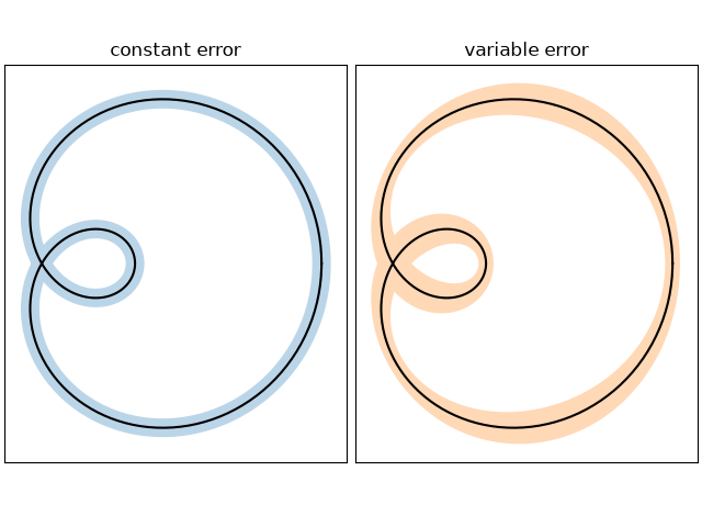
statistics/customized_violin
=========================
Source
"""
=========================
Violin plot customization
=========================
This example demonstrates how to fully customize violin plots. The first plot
shows the default style by providing only the data. The second plot first
limits what Matplotlib draws with additional keyword arguments. Then a
simplified representation of a box plot is drawn on top. Lastly, the styles of
the artists of the violins are modified.
For more information on violin plots, the scikit-learn docs have a great
section: https://scikit-learn.org/stable/modules/density.html
"""
import matplotlib.pyplot as plt
import numpy as np
def adjacent_values(vals, q1, q3):
upper_adjacent_value = q3 + (q3 - q1) * 1.5
upper_adjacent_value = np.clip(upper_adjacent_value, q3, vals[-1])
lower_adjacent_value = q1 - (q3 - q1) * 1.5
lower_adjacent_value = np.clip(lower_adjacent_value, vals[0], q1)
return lower_adjacent_value, upper_adjacent_value
def set_axis_style(ax, labels):
ax.set_xticks(np.arange(1, len(labels) + 1), labels=labels)
ax.set_xlim(0.25, len(labels) + 0.75)
ax.set_xlabel('Sample name')
# create test data
np.random.seed(19680801)
data = [sorted(np.random.normal(0, std, 100)) for std in range(1, 5)]
fig, (ax1, ax2, ax3) = plt.subplots(nrows=1, ncols=3, figsize=(9, 3), sharey=True)
ax1.set_title('Default violin plot')
ax1.set_ylabel('Observed values')
ax1.violinplot(data)
ax2.set_title('Set colors of violins')
ax2.set_ylabel('Observed values')
ax2.violinplot(
data,
facecolor=[('yellow', 0.3), ('blue', 0.3), ('red', 0.3), ('green', 0.3)],
linecolor='black',
)
# Note that when passing a sequence of colors, the method will repeat the sequence if
# less colors are provided than data distributions.
ax3.set_title('Customized violin plot')
parts = ax3.violinplot(
data, showmeans=False, showmedians=False, showextrema=False,
facecolor='#D43F3A', linecolor='black')
for pc in parts['bodies']:
pc.set_edgecolor('black')
pc.set_linewidth(1)
pc.set_alpha(1)
quartile1, medians, quartile3 = np.percentile(data, [25, 50, 75], axis=1)
whiskers = np.array([
adjacent_values(sorted_array, q1, q3)
for sorted_array, q1, q3 in zip(data, quartile1, quartile3)])
whiskers_min, whiskers_max = whiskers[:, 0], whiskers[:, 1]
inds = np.arange(1, len(medians) + 1)
ax3.scatter(inds, medians, marker='o', color='white', s=30, zorder=3)
ax3.vlines(inds, quartile1, quartile3, color='k', linestyle='-', lw=5)
ax3.vlines(inds, whiskers_min, whiskers_max, color='k', linestyle='-', lw=1)
# set style for the axes
labels = ['A', 'B', 'C', 'D']
for ax in [ax1, ax2, ax3]:
set_axis_style(ax, labels)
plt.subplots_adjust(bottom=0.15, wspace=0.05)
plt.show()
# %%
#
# .. tags:: plot-type: violin, domain: statistics
#
# .. admonition:: References
#
# The use of the following functions, methods, classes and modules is shown
# in this example:
#
# - `matplotlib.axes.Axes.violinplot` / `matplotlib.pyplot.violinplot`
# - `matplotlib.axes.Axes.vlines` / `matplotlib.pyplot.vlines`
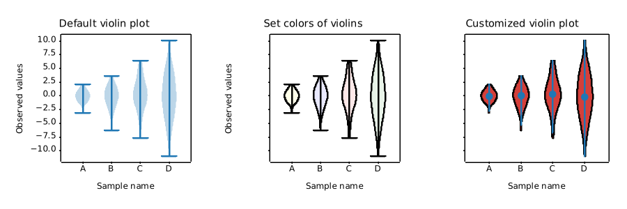
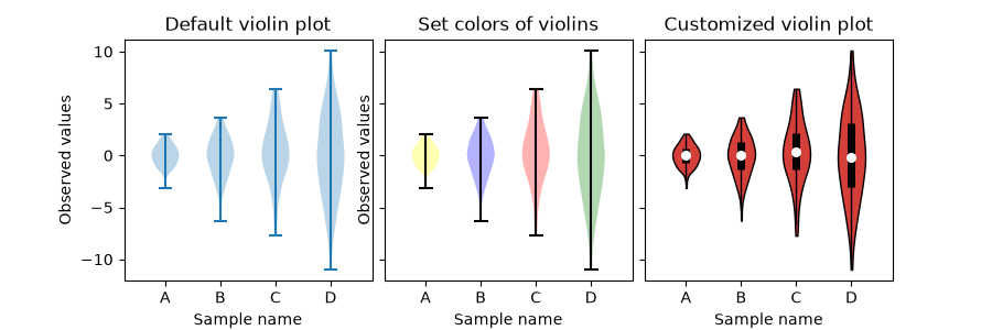
statistics/errorbar
=================
Source
""" ================= Errorbar function ================= This exhibits the most basic use of the error bar method. In this case, constant values are provided for the error in both the x- and y-directions. """ import matplotlib.pyplot as plt import numpy as np # example data x = np.arange(0.1, 4, 0.5) y = np.exp(-x) fig, ax = plt.subplots() ax.errorbar(x, y, xerr=0.2, yerr=0.4) plt.show() # %% # # # .. tags:: plot-type: errorbar, domain: statistics, # # .. admonition:: References # # The use of the following functions, methods, classes and modules is shown # in this example: # # - `matplotlib.axes.Axes.errorbar` / `matplotlib.pyplot.errorbar`
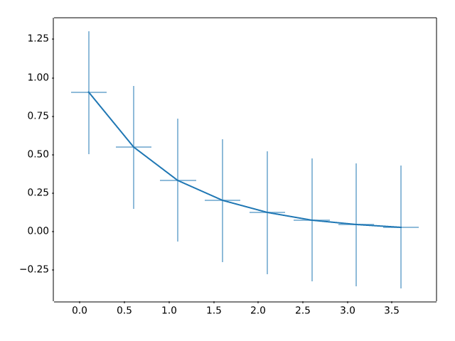
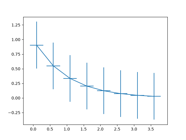
statistics/errorbar_features
=======================================
Source
"""
=======================================
Different ways of specifying error bars
=======================================
Errors can be specified as a constant value (as shown in
:doc:`/gallery/statistics/errorbar`). However, this example demonstrates
how they vary by specifying arrays of error values.
If the raw ``x`` and ``y`` data have length N, there are two options:
Array of shape (N,):
Error varies for each point, but the error values are
symmetric (i.e. the lower and upper values are equal).
Array of shape (2, N):
Error varies for each point, and the lower and upper limits
(in that order) are different (asymmetric case)
In addition, this example demonstrates how to use log
scale with error bars.
"""
import matplotlib.pyplot as plt
import numpy as np
# example data
x = np.arange(0.1, 4, 0.5)
y = np.exp(-x)
# example error bar values that vary with x-position
error = 0.1 + 0.2 * x
fig, (ax0, ax1) = plt.subplots(nrows=2, sharex=True)
ax0.errorbar(x, y, yerr=error, fmt='-o')
ax0.set_title('variable, symmetric error')
# error bar values w/ different -/+ errors that
# also vary with the x-position
lower_error = 0.4 * error
upper_error = error
asymmetric_error = [lower_error, upper_error]
ax1.errorbar(x, y, xerr=asymmetric_error, fmt='o')
ax1.set_title('variable, asymmetric error')
ax1.set_yscale('log')
plt.show()
# %%
#
# .. tags:: plot-type: errorbar, domain: statistics
#
# .. admonition:: References
#
# The use of the following functions, methods, classes and modules is shown
# in this example:
#
# - `matplotlib.axes.Axes.errorbar` / `matplotlib.pyplot.errorbar`
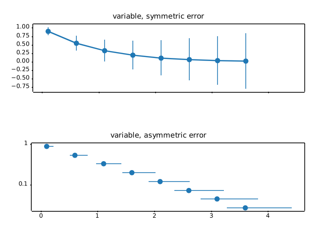
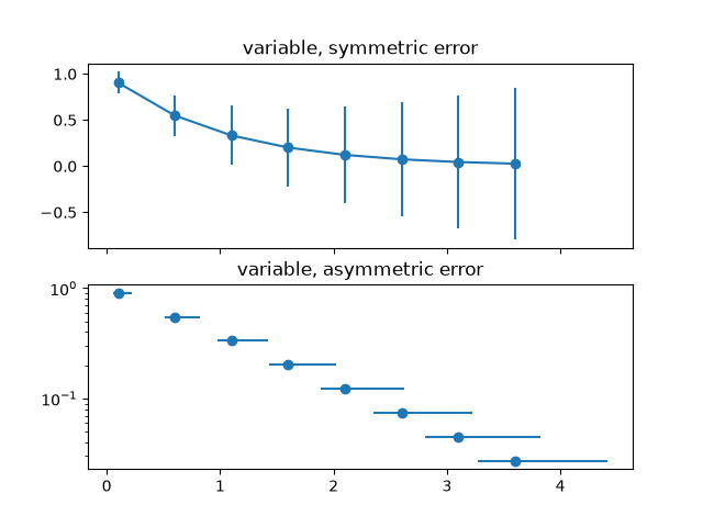
statistics/errorbar_limits
==============================================
Source
"""
==============================================
Including upper and lower limits in error bars
==============================================
In matplotlib, errors bars can have "limits". Applying limits to the
error bars essentially makes the error unidirectional. Because of that,
upper and lower limits can be applied in both the y- and x-directions
via the ``uplims``, ``lolims``, ``xuplims``, and ``xlolims`` parameters,
respectively. These parameters can be scalar or boolean arrays.
For example, if ``xlolims`` is ``True``, the x-error bars will only
extend from the data towards increasing values. If ``uplims`` is an
array filled with ``False`` except for the 4th and 7th values, all of the
y-error bars will be bidirectional, except the 4th and 7th bars, which
will extend from the data towards decreasing y-values.
"""
import matplotlib.pyplot as plt
import numpy as np
# example data
x = np.array([0.5, 1.0, 1.5, 2.0, 2.5, 3.0, 3.5, 4.0, 4.5, 5.0])
y = np.exp(-x)
xerr = 0.1
yerr = 0.2
# lower & upper limits of the error
lolims = np.array([0, 0, 1, 0, 1, 0, 0, 0, 1, 0], dtype=bool)
uplims = np.array([0, 1, 0, 0, 0, 1, 0, 0, 0, 1], dtype=bool)
ls = 'dotted'
fig, ax = plt.subplots(figsize=(7, 4))
# standard error bars
ax.errorbar(x, y, xerr=xerr, yerr=yerr, linestyle=ls)
# including upper limits
ax.errorbar(x, y + 0.5, xerr=xerr, yerr=yerr, uplims=uplims,
linestyle=ls)
# including lower limits
ax.errorbar(x, y + 1.0, xerr=xerr, yerr=yerr, lolims=lolims,
linestyle=ls)
# including upper and lower limits
ax.errorbar(x, y + 1.5, xerr=xerr, yerr=yerr,
lolims=lolims, uplims=uplims,
marker='o', markersize=8,
linestyle=ls)
# Plot a series with lower and upper limits in both x & y
# constant x-error with varying y-error
xerr = 0.2
yerr = np.full_like(x, 0.2)
yerr[[3, 6]] = 0.3
# mock up some limits by modifying previous data
xlolims = lolims
xuplims = uplims
lolims = np.zeros_like(x)
uplims = np.zeros_like(x)
lolims[[6]] = True # only limited at this index
uplims[[3]] = True # only limited at this index
# do the plotting
ax.errorbar(x, y + 2.1, xerr=xerr, yerr=yerr,
xlolims=xlolims, xuplims=xuplims,
uplims=uplims, lolims=lolims,
marker='o', markersize=8,
linestyle='none')
# tidy up the figure
ax.set_xlim(0, 5.5)
ax.set_title('Errorbar upper and lower limits')
plt.show()
# %%
#
# .. tags:: plot-type: errorbar, domain: statistics
#
# .. admonition:: References
#
# The use of the following functions, methods, classes and modules is shown
# in this example:
#
# - `matplotlib.axes.Axes.errorbar` / `matplotlib.pyplot.errorbar`
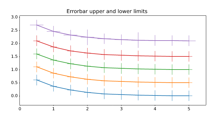
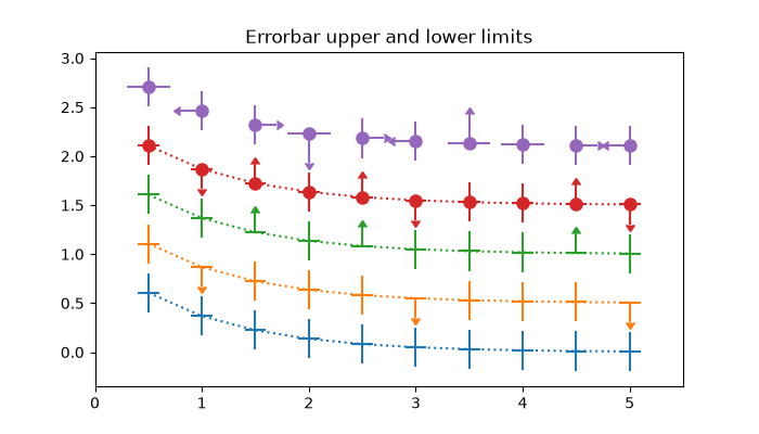
statistics/errorbar_limits_simple
========================
Source
"""
========================
Errorbar limit selection
========================
Illustration of selectively drawing lower and/or upper limit symbols on
errorbars using the parameters ``uplims``, ``lolims`` of `~.pyplot.errorbar`.
Alternatively, you can use 2xN values to draw errorbars in only one direction.
.. redirect-from:: /gallery/lines_bars_and_markers/errorbar_limits_simple
"""
import matplotlib.pyplot as plt
import numpy as np
fig = plt.figure()
x = np.arange(10)
y = 2.5 * np.sin(x / 20 * np.pi)
yerr = np.linspace(0.05, 0.2, 10)
plt.errorbar(x, y + 3, yerr=yerr, label='both limits (default)')
plt.errorbar(x, y + 2, yerr=yerr, uplims=True, label='uplims=True')
plt.errorbar(x, y + 1, yerr=yerr, uplims=True, lolims=True,
label='uplims=True, lolims=True')
upperlimits = [True, False] * 5
lowerlimits = [False, True] * 5
plt.errorbar(x, y, yerr=yerr, uplims=upperlimits, lolims=lowerlimits,
label='subsets of uplims and lolims')
plt.legend(loc='lower right')
# %%
# Similarly ``xuplims`` and ``xlolims`` can be used on the horizontal ``xerr``
# errorbars.
fig = plt.figure()
x = np.arange(10) / 10
y = (x + 0.1)**2
plt.errorbar(x, y, xerr=0.1, xlolims=True, label='xlolims=True')
y = (x + 0.1)**3
plt.errorbar(x + 0.6, y, xerr=0.1, xuplims=upperlimits, xlolims=lowerlimits,
label='subsets of xuplims and xlolims')
y = (x + 0.1)**4
plt.errorbar(x + 1.2, y, xerr=0.1, xuplims=True, label='xuplims=True')
plt.legend()
plt.show()
# %%
#
# .. admonition:: References
#
# The use of the following functions, methods, classes and modules is shown
# in this example:
#
# - `matplotlib.axes.Axes.errorbar` / `matplotlib.pyplot.errorbar`
#
# .. tags::
#
# component: error
# plot-type: errorbar
# level: beginner
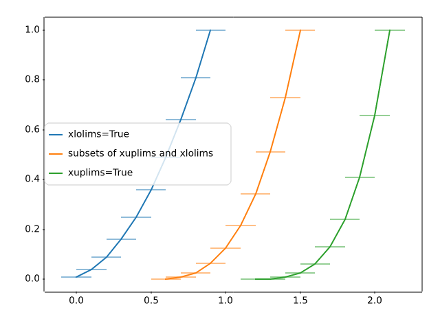
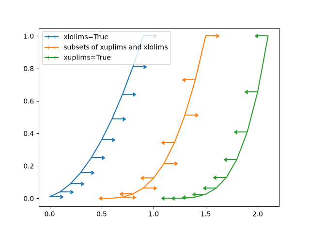
statistics/errorbar_subsample
====================
Source
"""
====================
Errorbar subsampling
====================
The parameter *errorevery* of `.Axes.errorbar` can be used to draw error bars
only on a subset of data points. This is particularly useful if there are many
data points with similar errors.
.. redirect-from:: /gallery/lines_bars_and_markers/errorbar_subsample
"""
import matplotlib.pyplot as plt
import numpy as np
# example data
x = np.arange(0.1, 4, 0.1)
y1 = np.exp(-1.0 * x)
y2 = np.exp(-0.5 * x)
# example variable error bar values
y1err = 0.1 + 0.1 * np.sqrt(x)
y2err = 0.1 + 0.1 * np.sqrt(x/2)
fig, (ax0, ax1, ax2) = plt.subplots(nrows=1, ncols=3, sharex=True,
figsize=(12, 6))
ax0.set_title('all errorbars')
ax0.errorbar(x, y1, yerr=y1err)
ax0.errorbar(x, y2, yerr=y2err)
ax1.set_title('only every 6th errorbar')
ax1.errorbar(x, y1, yerr=y1err, errorevery=6)
ax1.errorbar(x, y2, yerr=y2err, errorevery=6)
ax2.set_title('second series shifted by 3')
ax2.errorbar(x, y1, yerr=y1err, errorevery=(0, 6))
ax2.errorbar(x, y2, yerr=y2err, errorevery=(3, 6))
fig.suptitle('Errorbar subsampling')
plt.show()
# %%
# .. tags::
#
# component: error
# plot-type: errorbar
# level: beginner
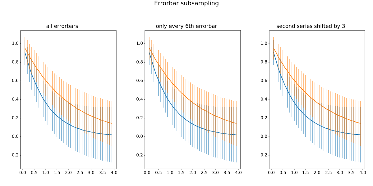
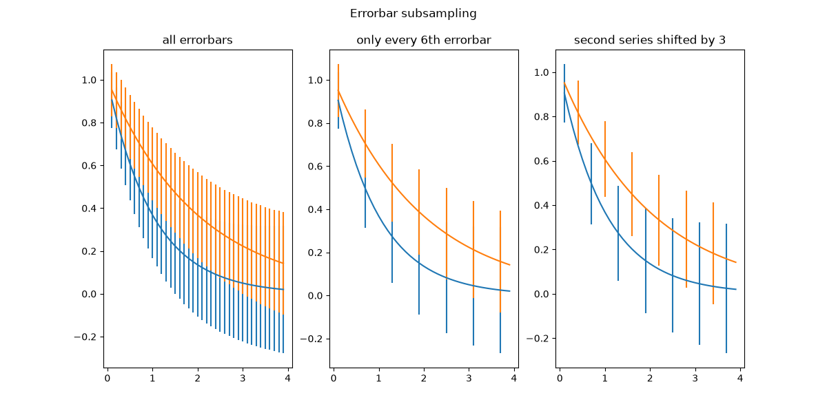
statistics/errorbars_and_boxes
==================================================
Source
"""
==================================================
Create boxes from error bars using PatchCollection
==================================================
In this example, we snazz up a pretty standard error bar plot by adding
a rectangle patch defined by the limits of the bars in both the x- and
y- directions. To do this, we have to write our own custom function
called ``make_error_boxes``. Close inspection of this function will
reveal the preferred pattern in writing functions for matplotlib:
1. an `~.axes.Axes` object is passed directly to the function
2. the function operates on the ``Axes`` methods directly, not through
the ``pyplot`` interface
3. plotting keyword arguments that could be abbreviated are spelled out for
better code readability in the future (for example we use *facecolor*
instead of *fc*)
4. the artists returned by the ``Axes`` plotting methods are then
returned by the function so that, if desired, their styles
can be modified later outside of the function (they are not
modified in this example).
"""
import matplotlib.pyplot as plt
import numpy as np
from matplotlib.collections import PatchCollection
from matplotlib.patches import Rectangle
# Number of data points
n = 5
# Dummy data
np.random.seed(19680801)
x = np.arange(0, n, 1)
y = np.random.rand(n) * 5.
# Dummy errors (above and below)
xerr = np.random.rand(2, n) + 0.1
yerr = np.random.rand(2, n) + 0.2
def make_error_boxes(ax, xdata, ydata, xerror, yerror, facecolor='r',
edgecolor='none', alpha=0.5):
# Loop over data points; create box from errors at each point
errorboxes = [Rectangle((x - xe[0], y - ye[0]), xe.sum(), ye.sum())
for x, y, xe, ye in zip(xdata, ydata, xerror.T, yerror.T)]
# Create patch collection with specified colour/alpha
pc = PatchCollection(errorboxes, facecolor=facecolor, alpha=alpha,
edgecolor=edgecolor)
# Add collection to Axes
ax.add_collection(pc)
# Plot errorbars
artists = ax.errorbar(xdata, ydata, xerr=xerror, yerr=yerror,
fmt='none', ecolor='k')
return artists
# Create figure and Axes
fig, ax = plt.subplots(1)
# Call function to create error boxes
_ = make_error_boxes(ax, x, y, xerr, yerr)
plt.show()
# %%
#
#
# .. tags::
#
# plot-type: errorbar
# component: rectangle
# component: patchcollection
# domain: statistics
#
# .. admonition:: References
#
# The use of the following functions, methods, classes and modules is shown
# in this example:
#
# - `matplotlib.axes.Axes.errorbar` / `matplotlib.pyplot.errorbar`
# - `matplotlib.axes.Axes.add_collection`
# - `matplotlib.collections.PatchCollection`
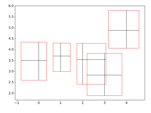
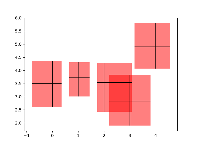
statistics/hexbin_demo
=====================
Source
"""
=====================
Hexagonal binned plot
=====================
`~.Axes.hexbin` is a 2D histogram plot, in which the bins are hexagons and
the color represents the number of data points within each bin.
"""
import matplotlib.pyplot as plt
import numpy as np
# Fixing random state for reproducibility
np.random.seed(19680801)
n = 100_000
x = np.random.standard_normal(n)
y = 2.0 + 3.0 * x + 4.0 * np.random.standard_normal(n)
xlim = x.min(), x.max()
ylim = y.min(), y.max()
fig, (ax0, ax1) = plt.subplots(ncols=2, sharey=True, figsize=(9, 4))
hb = ax0.hexbin(x, y, gridsize=50, cmap='inferno')
ax0.set(xlim=xlim, ylim=ylim)
ax0.set_title("Hexagon binning")
cb = fig.colorbar(hb, ax=ax0, label='counts')
hb = ax1.hexbin(x, y, gridsize=50, bins='log', cmap='inferno')
ax1.set(xlim=xlim, ylim=ylim)
ax1.set_title("With a log color scale")
cb = fig.colorbar(hb, ax=ax1, label='counts')
plt.show()
# %%
#
# .. tags:: plot-type: histogram, plot-type: hexbin, domain: statistics
#
# .. admonition:: References
#
# The use of the following functions, methods, classes and modules is shown
# in this example:
#
# - `matplotlib.axes.Axes.hexbin` / `matplotlib.pyplot.hexbin`
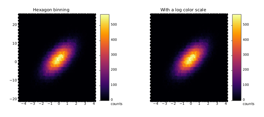
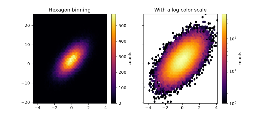
statistics/hist
==========
Source
"""
==========
Histograms
==========
How to plot histograms with Matplotlib.
"""
import matplotlib.pyplot as plt
import numpy as np
from matplotlib import colors
from matplotlib.ticker import PercentFormatter
# Create a random number generator with a fixed seed for reproducibility
rng = np.random.default_rng(19680801)
# %%
# Generate data and plot a simple histogram
# -----------------------------------------
#
# To generate a 1D histogram we only need a single vector of numbers. For a 2D
# histogram we'll need a second vector. We'll generate both below, and show
# the histogram for each vector.
N_points = 100000
n_bins = 20
# Generate two normal distributions
dist1 = rng.standard_normal(N_points)
dist2 = 0.4 * rng.standard_normal(N_points) + 5
fig, axs = plt.subplots(1, 2, sharey=True, tight_layout=True)
# We can set the number of bins with the *bins* keyword argument.
axs[0].hist(dist1, bins=n_bins)
axs[1].hist(dist2, bins=n_bins)
plt.show()
# %%
# Updating histogram colors
# -------------------------
#
# The histogram method returns (among other things) a ``patches`` object. This
# gives us access to the properties of the objects drawn. Using this, we can
# edit the histogram to our liking. Let's change the color of each bar
# based on its y value.
fig, axs = plt.subplots(1, 2, tight_layout=True)
# N is the count in each bin, bins is the lower-limit of the bin
N, bins, patches = axs[0].hist(dist1, bins=n_bins)
# We'll color code by height, but you could use any scalar
fracs = N / N.max()
# we need to normalize the data to 0..1 for the full range of the colormap
norm = colors.Normalize(fracs.min(), fracs.max())
# Now, we'll loop through our objects and set the color of each accordingly
for thisfrac, thispatch in zip(fracs, patches):
color = plt.colormaps["viridis"](norm(thisfrac))
thispatch.set_facecolor(color)
# We can also normalize our inputs by the total number of counts
axs[1].hist(dist1, bins=n_bins, density=True)
# Now we format the y-axis to display percentage
axs[1].yaxis.set_major_formatter(PercentFormatter(xmax=1))
# %%
# Plot a 2D histogram
# -------------------
#
# To plot a 2D histogram, one only needs two vectors of the same length,
# corresponding to each axis of the histogram.
fig, ax = plt.subplots(tight_layout=True)
hist = ax.hist2d(dist1, dist2)
# %%
# Customizing your histogram
# --------------------------
#
# Customizing a 2D histogram is similar to the 1D case, you can control
# visual components such as the bin size or color normalization.
fig, axs = plt.subplots(3, 1, figsize=(5, 15), sharex=True, sharey=True,
tight_layout=True)
# We can increase the number of bins on each axis
axs[0].hist2d(dist1, dist2, bins=40)
# As well as define normalization of the colors
axs[1].hist2d(dist1, dist2, bins=40, norm=colors.LogNorm())
# We can also define custom numbers of bins for each axis
axs[2].hist2d(dist1, dist2, bins=(80, 10), norm=colors.LogNorm())
# %%
#
# .. tags::
#
# plot-type: histogram,
# plot-type: histogram2d
# domain: statistics
# styling: color,
# component: normalization
# component: patch
#
# .. admonition:: References
#
# The use of the following functions, methods, classes and modules is shown
# in this example:
#
# - `matplotlib.axes.Axes.hist` / `matplotlib.pyplot.hist`
# - `matplotlib.pyplot.hist2d`
# - `matplotlib.ticker.PercentFormatter`
statistics/histogram_bihistogram
===========
Source
"""
===========
Bihistogram
===========
How to plot a bihistogram with Matplotlib.
"""
import matplotlib.pyplot as plt
import numpy as np
# Create a random number generator with a fixed seed for reproducibility
rng = np.random.default_rng(19680801)
# %%
# Generate data and plot a bihistogram
# ------------------------------------
#
# To generate a bihistogram we need two datasets (each being a vector of numbers).
# We will plot both histograms using plt.hist() and set the weights of the second
# one to be negative. We'll generate data below and plot the bihistogram.
N_points = 10_000
# Generate two normal distributions
dataset1 = np.random.normal(0, 1, size=N_points)
dataset2 = np.random.normal(1, 2, size=N_points)
# Use a constant bin width to make the two histograms easier to compare visually
bin_width = 0.25
bins = np.arange(np.min([dataset1, dataset2]),
np.max([dataset1, dataset2]) + bin_width, bin_width)
fig, ax = plt.subplots()
# Plot the first histogram
ax.hist(dataset1, bins=bins, label="Dataset 1")
# Plot the second histogram
# (notice the negative weights, which flip the histogram upside down)
ax.hist(dataset2, weights=-np.ones_like(dataset2), bins=bins, label="Dataset 2")
ax.axhline(0, color="k")
ax.legend()
plt.show()
# %%
#
# .. tags:: plot-type: histogram, domain: statistics, purpose: showcase
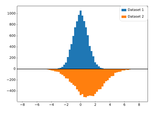
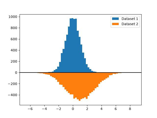
statistics/histogram_cumulative
========================
Source
"""
========================
Cumulative distributions
========================
This example shows how to plot the empirical cumulative distribution function
(ECDF) of a sample. We also show the theoretical CDF.
In engineering, ECDFs are sometimes called "non-exceedance" curves: the y-value
for a given x-value gives probability that an observation from the sample is
below that x-value. For example, the value of 220 on the x-axis corresponds to
about 0.80 on the y-axis, so there is an 80% chance that an observation in the
sample does not exceed 220. Conversely, the empirical *complementary*
cumulative distribution function (the ECCDF, or "exceedance" curve) shows the
probability y that an observation from the sample is above a value x.
A direct method to plot ECDFs is `.Axes.ecdf`. Passing ``complementary=True``
results in an ECCDF instead.
Alternatively, one can use ``ax.hist(data, density=True, cumulative=True)`` to
first bin the data, as if plotting a histogram, and then compute and plot the
cumulative sums of the frequencies of entries in each bin. Here, to plot the
ECCDF, pass ``cumulative=-1``. Note that this approach results in an
approximation of the E(C)CDF, whereas `.Axes.ecdf` is exact.
"""
import matplotlib.pyplot as plt
import numpy as np
np.random.seed(19680801)
mu = 200
sigma = 25
n_bins = 25
data = np.random.normal(mu, sigma, size=100)
fig = plt.figure(figsize=(9, 4), layout="constrained")
axs = fig.subplots(1, 2, sharex=True, sharey=True)
# Cumulative distributions.
axs[0].ecdf(data, label="CDF")
n, bins, patches = axs[0].hist(data, n_bins, density=True, histtype="step",
cumulative=True, label="Cumulative histogram")
x = np.linspace(data.min(), data.max())
y = ((1 / (np.sqrt(2 * np.pi) * sigma)) *
np.exp(-0.5 * (1 / sigma * (x - mu))**2))
y = y.cumsum()
y /= y[-1]
axs[0].plot(x, y, "k--", linewidth=1.5, label="Theory")
# Complementary cumulative distributions.
axs[1].ecdf(data, complementary=True, label="CCDF")
axs[1].hist(data, bins=bins, density=True, histtype="step", cumulative=-1,
label="Reversed cumulative histogram")
axs[1].plot(x, 1 - y, "k--", linewidth=1.5, label="Theory")
# Label the figure.
fig.suptitle("Cumulative distributions")
for ax in axs:
ax.grid(True)
ax.legend()
ax.set_xlabel("Annual rainfall (mm)")
ax.set_ylabel("Probability of occurrence")
ax.label_outer()
plt.show()
# %%
#
# .. tags:: plot-type: ecdf, plot-type: histogram, domain: statistics
#
# .. admonition:: References
#
# The use of the following functions, methods, classes and modules is shown
# in this example:
#
# - `matplotlib.axes.Axes.hist` / `matplotlib.pyplot.hist`
# - `matplotlib.axes.Axes.ecdf` / `matplotlib.pyplot.ecdf`
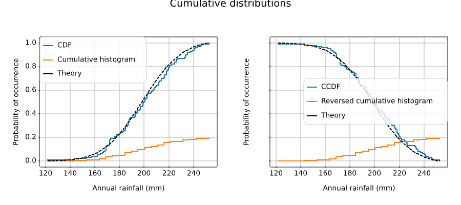
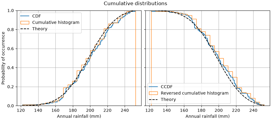
statistics/histogram_histtypes
================================================================
Source
"""
================================================================
Demo of the histogram function's different ``histtype`` settings
================================================================
* Histogram with step curve that has a color fill.
* Histogram with step curve with no fill.
* Histogram with custom and unequal bin widths.
* Two histograms with stacked bars.
Selecting different bin counts and sizes can significantly affect the
shape of a histogram. The Astropy docs have a great section on how to
select these parameters:
http://docs.astropy.org/en/stable/visualization/histogram.html
"""
import matplotlib.pyplot as plt
import numpy as np
np.random.seed(19680801)
mu_x = 200
sigma_x = 25
x = np.random.normal(mu_x, sigma_x, size=100)
mu_w = 200
sigma_w = 10
w = np.random.normal(mu_w, sigma_w, size=100)
fig, axs = plt.subplots(nrows=2, ncols=2)
axs[0, 0].hist(x, 20, density=True, histtype='stepfilled', facecolor='g',
alpha=0.75)
axs[0, 0].set_title('stepfilled')
axs[0, 1].hist(x, 20, density=True, histtype='step', facecolor='g',
alpha=0.75)
axs[0, 1].set_title('step')
axs[1, 0].hist(x, density=True, histtype='barstacked', rwidth=0.8)
axs[1, 0].hist(w, density=True, histtype='barstacked', rwidth=0.8)
axs[1, 0].set_title('barstacked')
# Create a histogram by providing the bin edges (unequally spaced).
bins = [100, 150, 180, 195, 205, 220, 250, 300]
axs[1, 1].hist(x, bins, density=True, histtype='bar', rwidth=0.8)
axs[1, 1].set_title('bar, unequal bins')
fig.tight_layout()
plt.show()
# %%
#
# .. tags:: plot-type: histogram, domain: statistics, purpose: reference
#
# .. admonition:: References
#
# The use of the following functions, methods, classes and modules is shown
# in this example:
#
# - `matplotlib.axes.Axes.hist` / `matplotlib.pyplot.hist`
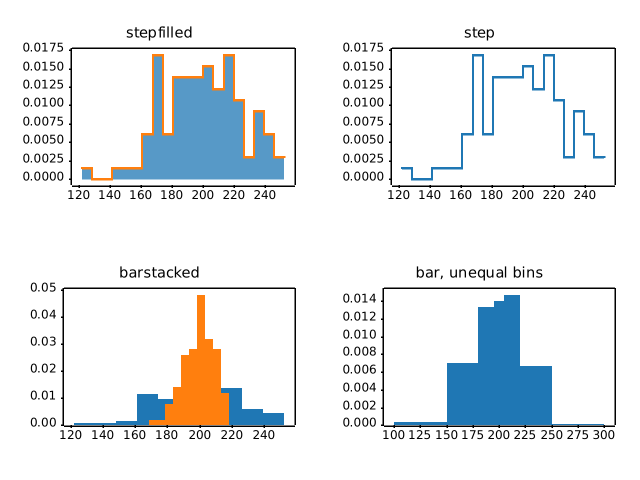
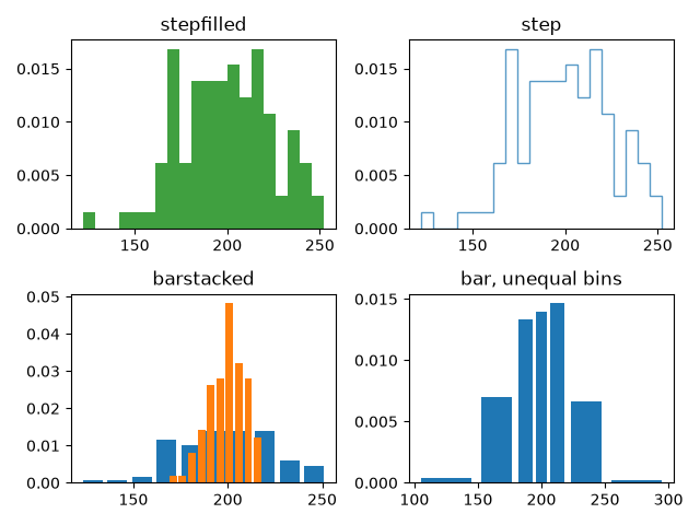
statistics/histogram_multihist
=====================================================
Source
"""
=====================================================
The histogram (hist) function with multiple data sets
=====================================================
Plot histogram with multiple sample sets and demonstrate:
* Use of legend with multiple sample sets
* Stacked bars
* Step curve with no fill
* Data sets of different sample sizes
Selecting different bin counts and sizes can significantly affect the
shape of a histogram. The Astropy docs have a great section on how to
select these parameters:
http://docs.astropy.org/en/stable/visualization/histogram.html
.. redirect-from:: /gallery/lines_bars_and_markers/filled_step
"""
# %%
import matplotlib.pyplot as plt
import numpy as np
np.random.seed(19680801)
n_bins = 10
x = np.random.randn(1000, 3)
fig, ((ax0, ax1), (ax2, ax3)) = plt.subplots(nrows=2, ncols=2)
colors = ['red', 'tan', 'lime']
ax0.hist(x, n_bins, density=True, histtype='bar', color=colors, label=colors)
ax0.legend(prop={'size': 10})
ax0.set_title('bars with legend')
ax1.hist(x, n_bins, density=True, histtype='bar', stacked=True)
ax1.set_title('stacked bar')
ax2.hist(x, n_bins, histtype='step', stacked=True, fill=False)
ax2.set_title('stack step (unfilled)')
# Make a multiple-histogram of data-sets with different length.
x_multi = [np.random.randn(n) for n in [10000, 5000, 2000]]
ax3.hist(x_multi, n_bins, histtype='bar')
ax3.set_title('different sample sizes')
fig.tight_layout()
plt.show()
# %%
# -----------------------------------
# Setting properties for each dataset
# -----------------------------------
#
# You can style the histograms individually by passing a list of values to the
# following parameters:
#
# * edgecolor
# * facecolor
# * hatch
# * linewidth
# * linestyle
#
#
# edgecolor
# .........
fig, ax = plt.subplots()
edgecolors = ['green', 'red', 'blue']
ax.hist(x, n_bins, fill=False, histtype="step", stacked=True,
edgecolor=edgecolors, label=edgecolors)
ax.legend()
ax.set_title('Stacked Steps with Edgecolors')
plt.show()
# %%
# facecolor
# .........
fig, ax = plt.subplots()
facecolors = ['green', 'red', 'blue']
ax.hist(x, n_bins, histtype="barstacked", facecolor=facecolors, label=facecolors)
ax.legend()
ax.set_title("Bars with different Facecolors")
plt.show()
# %%
# hatch
# .....
fig, ax = plt.subplots()
hatches = [".", "o", "x"]
ax.hist(x, n_bins, histtype="barstacked", hatch=hatches, label=hatches)
ax.legend()
ax.set_title("Hatches on Stacked Bars")
plt.show()
# %%
# linewidth
# .........
fig, ax = plt.subplots()
linewidths = [1, 2, 3]
edgecolors = ["green", "red", "blue"]
ax.hist(x, n_bins, fill=False, histtype="bar", linewidth=linewidths,
edgecolor=edgecolors, label=linewidths)
ax.legend()
ax.set_title("Bars with Linewidths")
plt.show()
# %%
# linestyle
# .........
fig, ax = plt.subplots()
linestyles = ['-', ':', '--']
ax.hist(x, n_bins, fill=False, histtype='bar', linestyle=linestyles,
edgecolor=edgecolors, label=linestyles)
ax.legend()
ax.set_title('Bars with Linestyles')
plt.show()
# %%
#
# .. tags:: plot-type: histogram, domain: statistics, purpose: reference
#
# .. admonition:: References
#
# The use of the following functions, methods, classes and modules is shown
# in this example:
#
# - `matplotlib.axes.Axes.hist` / `matplotlib.pyplot.hist`
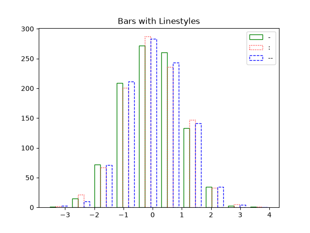
statistics/histogram_normalization
.. redirect-from:: /gallery/statistics/histogram_features
Source
"""
.. redirect-from:: /gallery/statistics/histogram_features
===================================
Histogram bins, density, and weight
===================================
The `.Axes.hist` method can flexibly create histograms in a few different ways,
which is flexible and helpful, but can also lead to confusion. In particular,
you can:
- bin the data as you want, either with an automatically chosen number of
bins, or with fixed bin edges,
- normalize the histogram so that its integral is one,
- and assign weights to the data points, so that each data point affects the
count in its bin differently.
The Matplotlib ``hist`` method calls `numpy.histogram` and plots the results,
therefore users should consult the numpy documentation for a definitive guide.
Histograms are created by defining bin edges, and taking a dataset of values
and sorting them into the bins, and counting or summing how much data is in
each bin. In this simple example, 9 numbers between 1 and 4 are sorted into 3
bins:
"""
import matplotlib.pyplot as plt
import numpy as np
rng = np.random.default_rng(19680801)
xdata = np.array([1.2, 2.3, 3.3, 3.1, 1.7, 3.4, 2.1, 1.25, 1.3])
xbins = np.array([1, 2, 3, 4])
# changing the style of the histogram bars just to make it
# very clear where the boundaries of the bins are:
style = {'facecolor': 'none', 'edgecolor': 'C0', 'linewidth': 3}
fig, ax = plt.subplots()
ax.hist(xdata, bins=xbins, **style)
# plot the xdata locations on the x axis:
ax.plot(xdata, 0*xdata, 'd')
ax.set_ylabel('Number per bin')
ax.set_xlabel('x bins (dx=1.0)')
# %%
# Modifying bins
# ==============
#
# Changing the bin size changes the shape of this sparse histogram, so its a
# good idea to choose bins with some care with respect to your data. Here we
# make the bins half as wide.
xbins = np.arange(1, 4.5, 0.5)
fig, ax = plt.subplots()
ax.hist(xdata, bins=xbins, **style)
ax.plot(xdata, 0*xdata, 'd')
ax.set_ylabel('Number per bin')
ax.set_xlabel('x bins (dx=0.5)')
# %%
# We can also let numpy (via Matplotlib) choose the bins automatically, or
# specify a number of bins to choose automatically:
fig, ax = plt.subplot_mosaic([['auto', 'n4']],
sharex=True, sharey=True, layout='constrained')
ax['auto'].hist(xdata, **style)
ax['auto'].plot(xdata, 0*xdata, 'd')
ax['auto'].set_ylabel('Number per bin')
ax['auto'].set_xlabel('x bins (auto)')
ax['n4'].hist(xdata, bins=4, **style)
ax['n4'].plot(xdata, 0*xdata, 'd')
ax['n4'].set_xlabel('x bins ("bins=4")')
# %%
# Normalizing histograms: density and weight
# ==========================================
#
# Counts-per-bin is the default length of each bar in the histogram. However,
# we can also normalize the bar lengths as a probability density function using
# the ``density`` parameter:
fig, ax = plt.subplots()
ax.hist(xdata, bins=xbins, density=True, **style)
ax.set_ylabel('Probability density [$V^{-1}$])')
ax.set_xlabel('x bins (dx=0.5 $V$)')
# %%
# This normalization can be a little hard to interpret when just exploring the
# data. The value attached to each bar is divided by the total number of data
# points *and* the width of the bin, and thus the values _integrate_ to one
# when integrating across the full range of data.
# e.g. ::
#
# density = counts / (sum(counts) * np.diff(bins))
# np.sum(density * np.diff(bins)) == 1
#
# This normalization is how `probability density functions
# <https://en.wikipedia.org/wiki/Probability_density_function>`_ are defined in
# statistics. If :math:`X` is a random variable on :math:`x`, then :math:`f_X`
# is is the probability density function if :math:`P[a<X<b] = \int_a^b f_X dx`.
# If the units of x are Volts, then the units of :math:`f_X` are :math:`V^{-1}`
# or probability per change in voltage.
#
# The usefulness of this normalization is a little more clear when we draw from
# a known distribution and try to compare with theory. So, choose 1000 points
# from a `normal distribution
# <https://en.wikipedia.org/wiki/Normal_distribution>`_, and also calculate the
# known probability density function:
xdata = rng.normal(size=1000)
xpdf = np.arange(-4, 4, 0.1)
pdf = 1 / (np.sqrt(2 * np.pi)) * np.exp(-xpdf**2 / 2)
# %%
# If we don't use ``density=True``, we need to scale the expected probability
# distribution function by both the length of the data and the width of the
# bins:
fig, ax = plt.subplot_mosaic([['False', 'True']], layout='constrained')
dx = 0.1
xbins = np.arange(-4, 4, dx)
ax['False'].hist(xdata, bins=xbins, density=False, histtype='step', label='Counts')
# scale and plot the expected pdf:
ax['False'].plot(xpdf, pdf * len(xdata) * dx, label=r'$N\,f_X(x)\,\delta x$')
ax['False'].set_ylabel('Count per bin')
ax['False'].set_xlabel('x bins [V]')
ax['False'].legend()
ax['True'].hist(xdata, bins=xbins, density=True, histtype='step', label='density')
ax['True'].plot(xpdf, pdf, label='$f_X(x)$')
ax['True'].set_ylabel('Probability density [$V^{-1}$]')
ax['True'].set_xlabel('x bins [$V$]')
ax['True'].legend()
# %%
# One advantage of using the density is therefore that the shape and amplitude
# of the histogram does not depend on the size of the bins. Consider an
# extreme case where the bins do not have the same width. In this example, the
# bins below ``x=-1.25`` are six times wider than the rest of the bins. By
# normalizing by density, we preserve the shape of the distribution, whereas if
# we do not, then the wider bins have much higher counts than the thinner bins:
fig, ax = plt.subplot_mosaic([['False', 'True']], layout='constrained')
dx = 0.1
xbins = np.hstack([np.arange(-4, -1.25, 6*dx), np.arange(-1.25, 4, dx)])
ax['False'].hist(xdata, bins=xbins, density=False, histtype='step', label='Counts')
ax['False'].plot(xpdf, pdf * len(xdata) * dx, label=r'$N\,f_X(x)\,\delta x_0$')
ax['False'].set_ylabel('Count per bin')
ax['False'].set_xlabel('x bins [V]')
ax['False'].legend()
ax['True'].hist(xdata, bins=xbins, density=True, histtype='step', label='density')
ax['True'].plot(xpdf, pdf, label='$f_X(x)$')
ax['True'].set_ylabel('Probability density [$V^{-1}$]')
ax['True'].set_xlabel('x bins [$V$]')
ax['True'].legend()
# %%
# Similarly, if we want to compare histograms with different bin widths, we may
# want to use ``density=True``:
fig, ax = plt.subplot_mosaic([['False', 'True']], layout='constrained')
# expected PDF
ax['True'].plot(xpdf, pdf, '--', label='$f_X(x)$', color='k')
for nn, dx in enumerate([0.1, 0.4, 1.2]):
xbins = np.arange(-4, 4, dx)
# expected histogram:
ax['False'].plot(xpdf, pdf*1000*dx, '--', color=f'C{nn}')
ax['False'].hist(xdata, bins=xbins, density=False, histtype='step')
ax['True'].hist(xdata, bins=xbins, density=True, histtype='step', label=dx)
# Labels:
ax['False'].set_xlabel('x bins [$V$]')
ax['False'].set_ylabel('Count per bin')
ax['True'].set_ylabel('Probability density [$V^{-1}$]')
ax['True'].set_xlabel('x bins [$V$]')
ax['True'].legend(fontsize='small', title='bin width:')
# %%
# Sometimes people want to normalize so that the sum of counts is one. This is
# analogous to a `probability mass function
# <https://en.wikipedia.org/wiki/Probability_mass_function>`_ for a discrete
# variable where the sum of probabilities for all the values equals one. Using
# ``hist``, we can get this normalization if we set the *weights* to 1/N.
# Note that the amplitude of this normalized histogram still depends on
# width and/or number of the bins:
fig, ax = plt.subplots(layout='constrained', figsize=(3.5, 3))
for nn, dx in enumerate([0.1, 0.4, 1.2]):
xbins = np.arange(-4, 4, dx)
ax.hist(xdata, bins=xbins, weights=1/len(xdata) * np.ones(len(xdata)),
histtype='step', label=f'{dx}')
ax.set_xlabel('x bins [$V$]')
ax.set_ylabel('Bin count / N')
ax.legend(fontsize='small', title='bin width:')
# %%
# The value of normalizing histograms is comparing two distributions that have
# different sized populations. Here we compare the distribution of ``xdata``
# with a population of 1000, and ``xdata2`` with 100 members.
xdata2 = rng.normal(size=100)
fig, ax = plt.subplot_mosaic([['no_norm', 'density', 'weight']],
layout='constrained', figsize=(8, 4))
xbins = np.arange(-4, 4, 0.25)
ax['no_norm'].hist(xdata, bins=xbins, histtype='step')
ax['no_norm'].hist(xdata2, bins=xbins, histtype='step')
ax['no_norm'].set_ylabel('Counts')
ax['no_norm'].set_xlabel('x bins [$V$]')
ax['no_norm'].set_title('No normalization')
ax['density'].hist(xdata, bins=xbins, histtype='step', density=True)
ax['density'].hist(xdata2, bins=xbins, histtype='step', density=True)
ax['density'].set_ylabel('Probability density [$V^{-1}$]')
ax['density'].set_title('Density=True')
ax['density'].set_xlabel('x bins [$V$]')
ax['weight'].hist(xdata, bins=xbins, histtype='step',
weights=1 / len(xdata) * np.ones(len(xdata)),
label='N=1000')
ax['weight'].hist(xdata2, bins=xbins, histtype='step',
weights=1 / len(xdata2) * np.ones(len(xdata2)),
label='N=100')
ax['weight'].set_xlabel('x bins [$V$]')
ax['weight'].set_ylabel('Counts / N')
ax['weight'].legend(fontsize='small')
ax['weight'].set_title('Weight = 1/N')
plt.show()
# %%
#
# .. tags:: plot-type: histogram, domain: statistics
#
# .. admonition:: References
#
# The use of the following functions, methods, classes and modules is shown
# in this example:
#
# - `matplotlib.axes.Axes.hist` / `matplotlib.pyplot.hist`
# - `matplotlib.axes.Axes.set_title`
# - `matplotlib.axes.Axes.set_xlabel`
# - `matplotlib.axes.Axes.set_ylabel`
# - `matplotlib.axes.Axes.legend`
statistics/multiple_histograms_side_by_side
================================
Source
"""
================================
Multiple histograms side by side
================================
This example plots horizontal histograms of different samples along
a categorical x-axis. Additionally, the histograms are plotted to
be symmetrical about their x-position, thus making them very similar
to violin plots.
To make this highly specialized plot, we can't use the standard ``hist``
method. Instead, we use ``barh`` to draw the horizontal bars directly. The
vertical positions and lengths of the bars are computed via the
``np.histogram`` function. The histograms for all the samples are
computed using the same range (min and max values) and number of bins,
so that the bins for each sample are in the same vertical positions.
Selecting different bin counts and sizes can significantly affect the
shape of a histogram. The Astropy docs have a great section on how to
select these parameters:
http://docs.astropy.org/en/stable/visualization/histogram.html
"""
import matplotlib.pyplot as plt
import numpy as np
np.random.seed(19680801)
number_of_bins = 20
# An example of three data sets to compare
number_of_data_points = 387
labels = ["A", "B", "C"]
data_sets = [np.random.normal(0, 1, number_of_data_points),
np.random.normal(6, 1, number_of_data_points),
np.random.normal(-3, 1, number_of_data_points)]
# Computed quantities to aid plotting
hist_range = (np.min(data_sets), np.max(data_sets))
binned_data_sets = [
np.histogram(d, range=hist_range, bins=number_of_bins)[0]
for d in data_sets
]
binned_maximums = np.max(binned_data_sets, axis=1)
x_locations = np.arange(0, sum(binned_maximums), np.max(binned_maximums))
# The bin_edges are the same for all of the histograms
bin_edges = np.linspace(hist_range[0], hist_range[1], number_of_bins + 1)
heights = np.diff(bin_edges)
centers = bin_edges[:-1] + heights / 2
# Cycle through and plot each histogram
fig, ax = plt.subplots()
for x_loc, binned_data in zip(x_locations, binned_data_sets):
lefts = x_loc - 0.5 * binned_data
ax.barh(centers, binned_data, height=heights, left=lefts)
ax.set_xticks(x_locations, labels)
ax.set_ylabel("Data values")
ax.set_xlabel("Data sets")
plt.show()
# %%
#
# .. tags::
#
# domain: statistics
# plot-type: barh
# plot-type: histogram
# styling: position
#
# .. admonition:: References
#
# The use of the following functions, methods, classes and modules is shown
# in this example:
#
# - `matplotlib.axes.Axes.barh` / `matplotlib.pyplot.barh`
statistics/psd_demo
============================
Source
"""
============================
Power spectral density (PSD)
============================
Plotting power spectral density (PSD) using `~.Axes.psd`.
The PSD is a common plot in the field of signal processing. NumPy has
many useful libraries for computing a PSD. Below we demo a few examples
of how this can be accomplished and visualized with Matplotlib.
.. redirect-from:: /gallery/lines_bars_and_markers/psd_demo
"""
import matplotlib.pyplot as plt
import numpy as np
import matplotlib.mlab as mlab
# Fixing random state for reproducibility
np.random.seed(19680801)
dt = 0.01
t = np.arange(0, 10, dt)
nse = np.random.randn(len(t))
r = np.exp(-t / 0.05)
cnse = np.convolve(nse, r) * dt
cnse = cnse[:len(t)]
s = 0.1 * np.sin(2 * np.pi * t) + cnse
fig, (ax0, ax1) = plt.subplots(2, 1, layout='constrained')
ax0.plot(t, s)
ax0.set_xlabel('Time (s)')
ax0.set_ylabel('Signal')
ax1.psd(s, NFFT=512, Fs=1 / dt)
plt.show()
# %%
# Compare this with the equivalent Matlab code to accomplish the same thing::
#
# dt = 0.01;
# t = [0:dt:10];
# nse = randn(size(t));
# r = exp(-t/0.05);
# cnse = conv(nse, r)*dt;
# cnse = cnse(1:length(t));
# s = 0.1*sin(2*pi*t) + cnse;
#
# subplot(211)
# plot(t, s)
# subplot(212)
# psd(s, 512, 1/dt)
#
# Below we'll show a slightly more complex example that demonstrates
# how padding affects the resulting PSD.
dt = np.pi / 100.
fs = 1. / dt
t = np.arange(0, 8, dt)
y = 10. * np.sin(2 * np.pi * 4 * t) + 5. * np.sin(2 * np.pi * 4.25 * t)
y = y + np.random.randn(*t.shape)
# Plot the raw time series
fig, axs = plt.subplot_mosaic([
['signal', 'signal', 'signal'],
['zero padding', 'block size', 'overlap'],
], layout='constrained')
axs['signal'].plot(t, y)
axs['signal'].set_xlabel('Time (s)')
axs['signal'].set_ylabel('Signal')
# Plot the PSD with different amounts of zero padding. This uses the entire
# time series at once
axs['zero padding'].psd(y, NFFT=len(t), pad_to=len(t), Fs=fs)
axs['zero padding'].psd(y, NFFT=len(t), pad_to=len(t) * 2, Fs=fs)
axs['zero padding'].psd(y, NFFT=len(t), pad_to=len(t) * 4, Fs=fs)
# Plot the PSD with different block sizes, Zero pad to the length of the
# original data sequence.
axs['block size'].psd(y, NFFT=len(t), pad_to=len(t), Fs=fs)
axs['block size'].psd(y, NFFT=len(t) // 2, pad_to=len(t), Fs=fs)
axs['block size'].psd(y, NFFT=len(t) // 4, pad_to=len(t), Fs=fs)
axs['block size'].set_ylabel('')
# Plot the PSD with different amounts of overlap between blocks
axs['overlap'].psd(y, NFFT=len(t) // 2, pad_to=len(t), noverlap=0, Fs=fs)
axs['overlap'].psd(y, NFFT=len(t) // 2, pad_to=len(t),
noverlap=int(0.025 * len(t)), Fs=fs)
axs['overlap'].psd(y, NFFT=len(t) // 2, pad_to=len(t),
noverlap=int(0.1 * len(t)), Fs=fs)
axs['overlap'].set_ylabel('')
axs['overlap'].set_title('overlap')
for title, ax in axs.items():
if title == 'signal':
continue
ax.set_title(title)
ax.sharex(axs['zero padding'])
ax.sharey(axs['zero padding'])
plt.show()
# %%
# This is a ported version of a MATLAB example from the signal
# processing toolbox that showed some difference at one time between
# Matplotlib's and MATLAB's scaling of the PSD.
fs = 1000
t = np.linspace(0, 0.3, 301)
A = np.array([2, 8]).reshape(-1, 1)
f = np.array([150, 140]).reshape(-1, 1)
xn = (A * np.sin(2 * np.pi * f * t)).sum(axis=0)
xn += 5 * np.random.randn(*t.shape)
fig, (ax0, ax1) = plt.subplots(ncols=2, layout='constrained')
yticks = np.arange(-50, 30, 10)
yrange = (yticks[0], yticks[-1])
xticks = np.arange(0, 550, 100)
ax0.psd(xn, NFFT=301, Fs=fs, window=mlab.window_none, pad_to=1024,
scale_by_freq=True)
ax0.set_title('Periodogram')
ax0.set_yticks(yticks)
ax0.set_xticks(xticks)
ax0.grid(True)
ax0.set_ylim(yrange)
ax1.psd(xn, NFFT=150, Fs=fs, window=mlab.window_none, pad_to=512, noverlap=75,
scale_by_freq=True)
ax1.set_title('Welch')
ax1.set_xticks(xticks)
ax1.set_yticks(yticks)
ax1.set_ylabel('') # overwrite the y-label added by `psd`
ax1.grid(True)
ax1.set_ylim(yrange)
plt.show()
# %%
# This is a ported version of a MATLAB example from the signal
# processing toolbox that showed some difference at one time between
# Matplotlib's and MATLAB's scaling of the PSD.
#
# It uses a complex signal so we can see that complex PSD's work properly.
prng = np.random.RandomState(19680801) # to ensure reproducibility
fs = 1000
t = np.linspace(0, 0.3, 301)
A = np.array([2, 8]).reshape(-1, 1)
f = np.array([150, 140]).reshape(-1, 1)
xn = (A * np.exp(2j * np.pi * f * t)).sum(axis=0) + 5 * prng.randn(*t.shape)
fig, (ax0, ax1) = plt.subplots(ncols=2, layout='constrained')
yticks = np.arange(-50, 30, 10)
yrange = (yticks[0], yticks[-1])
xticks = np.arange(-500, 550, 200)
ax0.psd(xn, NFFT=301, Fs=fs, window=mlab.window_none, pad_to=1024,
scale_by_freq=True)
ax0.set_title('Periodogram')
ax0.set_yticks(yticks)
ax0.set_xticks(xticks)
ax0.grid(True)
ax0.set_ylim(yrange)
ax1.psd(xn, NFFT=150, Fs=fs, window=mlab.window_none, pad_to=512, noverlap=75,
scale_by_freq=True)
ax1.set_title('Welch')
ax1.set_xticks(xticks)
ax1.set_yticks(yticks)
ax1.set_ylabel('') # overwrite the y-label added by `psd`
ax1.grid(True)
ax1.set_ylim(yrange)
plt.show()
# %%
# .. tags::
#
# domain: signal-processing
# plot-type: line
# level: intermediate
statistics/time_series_histogram
=====================
Source
"""
=====================
Time Series Histogram
=====================
This example demonstrates how to efficiently visualize large numbers of time
series in a way that could potentially reveal hidden substructure and patterns
that are not immediately obvious, and display them in a visually appealing way.
In this example, we generate multiple sinusoidal "signal" series that are
buried under a larger number of random walk "noise/background" series. For an
unbiased Gaussian random walk with standard deviation of σ, the RMS deviation
from the origin after n steps is σ*sqrt(n). So in order to keep the sinusoids
visible on the same scale as the random walks, we scale the amplitude by the
random walk RMS. In addition, we also introduce a small random offset ``phi``
to shift the sines left/right, and some additive random noise to shift
individual data points up/down to make the signal a bit more "realistic" (you
wouldn't expect a perfect sine wave to appear in your data).
The first plot shows the typical way of visualizing multiple time series by
overlaying them on top of each other with ``plt.plot`` and a small value of
``alpha``. The second and third plots show how to reinterpret the data as a 2d
histogram, with optional interpolation between data points, by using
``np.histogram2d`` and ``plt.pcolormesh``.
"""
import time
import matplotlib.pyplot as plt
import numpy as np
fig, axes = plt.subplots(nrows=3, figsize=(6, 8), layout='constrained')
# Fix random state for reproducibility
np.random.seed(19680801)
# Make some data; a 1D random walk + small fraction of sine waves
num_series = 1000
num_points = 100
SNR = 0.10 # Signal to Noise Ratio
x = np.linspace(0, 4 * np.pi, num_points)
# Generate unbiased Gaussian random walks
Y = np.cumsum(np.random.randn(num_series, num_points), axis=-1)
# Generate sinusoidal signals
num_signal = round(SNR * num_series)
phi = (np.pi / 8) * np.random.randn(num_signal, 1) # small random offset
Y[-num_signal:] = (
np.sqrt(np.arange(num_points)) # random walk RMS scaling factor
* (np.sin(x - phi)
+ 0.05 * np.random.randn(num_signal, num_points)) # small random noise
)
# Plot series using `plot` and a small value of `alpha`. With this view it is
# very difficult to observe the sinusoidal behavior because of how many
# overlapping series there are. It also takes a bit of time to run because so
# many individual artists need to be generated.
tic = time.time()
axes[0].plot(x, Y.T, color="C0", alpha=0.1)
toc = time.time()
axes[0].set_title("Line plot with alpha")
print(f"{toc-tic:.3f} sec. elapsed")
# Now we will convert the multiple time series into a histogram. Not only will
# the hidden signal be more visible, but it is also a much quicker procedure.
tic = time.time()
# Linearly interpolate between the points in each time series
num_fine = 800
x_fine = np.linspace(x.min(), x.max(), num_fine)
y_fine = np.concatenate([np.interp(x_fine, x, y_row) for y_row in Y])
x_fine = np.broadcast_to(x_fine, (num_series, num_fine)).ravel()
# Plot (x, y) points in 2d histogram with log colorscale
# It is pretty evident that there is some kind of structure under the noise
# You can tune vmax to make signal more visible
cmap = plt.colormaps["plasma"]
cmap = cmap.with_extremes(bad=cmap(0))
h, xedges, yedges = np.histogram2d(x_fine, y_fine, bins=[400, 100])
pcm = axes[1].pcolormesh(xedges, yedges, h.T, cmap=cmap,
norm="log", vmax=1.5e2, rasterized=True)
fig.colorbar(pcm, ax=axes[1], label="# points", pad=0)
axes[1].set_title("2d histogram and log color scale")
# Same data but on linear color scale
pcm = axes[2].pcolormesh(xedges, yedges, h.T, cmap=cmap,
vmax=1.5e2, rasterized=True)
fig.colorbar(pcm, ax=axes[2], label="# points", pad=0)
axes[2].set_title("2d histogram and linear color scale")
toc = time.time()
print(f"{toc-tic:.3f} sec. elapsed")
plt.show()
# %%
#
# .. tags::
#
# plot-type: histogram2d
# plot-type: pcolormesh
# purpose: storytelling
# styling: color
# styling: colormap
#
# .. admonition:: References
#
# The use of the following functions, methods, classes and modules is shown
# in this example:
#
# - `matplotlib.axes.Axes.pcolormesh` / `matplotlib.pyplot.pcolormesh`
# - `matplotlib.figure.Figure.colorbar`
AttributeError: 'str' object has no attribute 'vmin'
statistics/violinplot
==================
Source
"""
==================
Violin plot basics
==================
Violin plots are similar to histograms and box plots in that they show
an abstract representation of the probability distribution of the
sample. Rather than showing counts of data points that fall into bins
or order statistics, violin plots use kernel density estimation (KDE) to
compute an empirical distribution of the sample. That computation
is controlled by several parameters. This example demonstrates how to
modify the number of points at which the KDE is evaluated (``points``)
and how to modify the bandwidth of the KDE (``bw_method``).
For more information on violin plots and KDE, the scikit-learn docs
have a great section: https://scikit-learn.org/stable/modules/density.html
"""
import matplotlib.pyplot as plt
import numpy as np
# Fixing random state for reproducibility
np.random.seed(19680801)
# fake data
fs = 10 # fontsize
pos = [1, 2, 4, 5, 7, 8]
data = [np.random.normal(0, std, size=100) for std in pos]
fig, axs = plt.subplots(nrows=2, ncols=6, figsize=(10, 4))
axs[0, 0].violinplot(data, pos, points=20, widths=0.3,
showmeans=True, showextrema=True, showmedians=True)
axs[0, 0].set_title('Custom violin 1', fontsize=fs)
axs[0, 1].violinplot(data, pos, points=40, widths=0.5,
showmeans=True, showextrema=True, showmedians=True,
bw_method='silverman')
axs[0, 1].set_title('Custom violin 2', fontsize=fs)
axs[0, 2].violinplot(data, pos, points=60, widths=0.7, showmeans=True,
showextrema=True, showmedians=True, bw_method=0.5)
axs[0, 2].set_title('Custom violin 3', fontsize=fs)
axs[0, 3].violinplot(data, pos, points=60, widths=0.7, showmeans=True,
showextrema=True, showmedians=True, bw_method=0.5,
quantiles=[[0.1], [], [], [0.175, 0.954], [0.75], [0.25]])
axs[0, 3].set_title('Custom violin 4', fontsize=fs)
axs[0, 4].violinplot(data[-1:], pos[-1:], points=60, widths=0.7,
showmeans=True, showextrema=True, showmedians=True,
quantiles=[0.05, 0.1, 0.8, 0.9], bw_method=0.5)
axs[0, 4].set_title('Custom violin 5', fontsize=fs)
axs[0, 5].violinplot(data[-1:], pos[-1:], points=60, widths=0.7,
showmeans=True, showextrema=True, showmedians=True,
quantiles=[0.05, 0.1, 0.8, 0.9], bw_method=0.5, side='low')
axs[0, 5].violinplot(data[-1:], pos[-1:], points=60, widths=0.7,
showmeans=True, showextrema=True, showmedians=True,
quantiles=[0.05, 0.1, 0.8, 0.9], bw_method=0.5, side='high')
axs[0, 5].set_title('Custom violin 6', fontsize=fs)
axs[1, 0].violinplot(data, pos, points=80, orientation='horizontal', widths=0.7,
showmeans=True, showextrema=True, showmedians=True)
axs[1, 0].set_title('Custom violin 7', fontsize=fs)
axs[1, 1].violinplot(data, pos, points=100, orientation='horizontal', widths=0.9,
showmeans=True, showextrema=True, showmedians=True,
bw_method='silverman')
axs[1, 1].set_title('Custom violin 8', fontsize=fs)
axs[1, 2].violinplot(data, pos, points=200, orientation='horizontal', widths=1.1,
showmeans=True, showextrema=True, showmedians=True,
bw_method=0.5)
axs[1, 2].set_title('Custom violin 9', fontsize=fs)
axs[1, 3].violinplot(data, pos, points=200, orientation='horizontal', widths=1.1,
showmeans=True, showextrema=True, showmedians=True,
quantiles=[[0.1], [], [], [0.175, 0.954], [0.75], [0.25]],
bw_method=0.5)
axs[1, 3].set_title('Custom violin 10', fontsize=fs)
axs[1, 4].violinplot(data[-1:], pos[-1:], points=200, orientation='horizontal',
widths=1.1, showmeans=True, showextrema=True, showmedians=True,
quantiles=[0.05, 0.1, 0.8, 0.9], bw_method=0.5)
axs[1, 4].set_title('Custom violin 11', fontsize=fs)
axs[1, 5].violinplot(data[-1:], pos[-1:], points=200, orientation='horizontal',
widths=1.1, showmeans=True, showextrema=True, showmedians=True,
quantiles=[0.05, 0.1, 0.8, 0.9], bw_method=0.5, side='low')
axs[1, 5].violinplot(data[-1:], pos[-1:], points=200, orientation='horizontal',
widths=1.1, showmeans=True, showextrema=True, showmedians=True,
quantiles=[0.05, 0.1, 0.8, 0.9], bw_method=0.5, side='high')
axs[1, 5].set_title('Custom violin 12', fontsize=fs)
for ax in axs.flat:
ax.set_yticklabels([])
fig.suptitle("Violin Plotting Examples")
fig.subplots_adjust(hspace=0.4)
plt.show()
# %%
#
# .. tags:: plot-type: violin, domain: statistics
#
# .. admonition:: References
#
# The use of the following functions, methods, classes and modules is shown
# in this example:
#
# - `matplotlib.axes.Axes.violinplot` / `matplotlib.pyplot.violinplot`
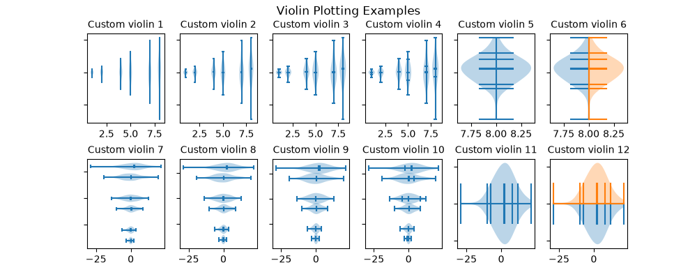
statistics/xcorr_acorr_demo
===========================
Source
"""
===========================
Cross- and auto-correlation
===========================
Example use of cross-correlation (`~.Axes.xcorr`) and auto-correlation
(`~.Axes.acorr`) plots.
.. redirect-from:: /gallery/lines_bars_and_markers/xcorr_acorr_demo
"""
import matplotlib.pyplot as plt
import numpy as np
# Fixing random state for reproducibility
np.random.seed(19680801)
x, y = np.random.randn(2, 100)
fig, [ax1, ax2] = plt.subplots(2, 1, sharex=True)
ax1.xcorr(x, y, usevlines=True, maxlags=50, normed=True, lw=2)
ax1.grid(True)
ax1.set_title('Cross-correlation (xcorr)')
ax2.acorr(x, usevlines=True, normed=True, maxlags=50, lw=2)
ax2.grid(True)
ax2.set_title('Auto-correlation (acorr)')
plt.show()
# %%
#
# .. admonition:: References
#
# The use of the following functions, methods, classes and modules is shown
# in this example:
#
# - `matplotlib.axes.Axes.acorr` / `matplotlib.pyplot.acorr`
# - `matplotlib.axes.Axes.xcorr` / `matplotlib.pyplot.xcorr`
#
# .. tags::
#
# domain: statistics
# level: beginner
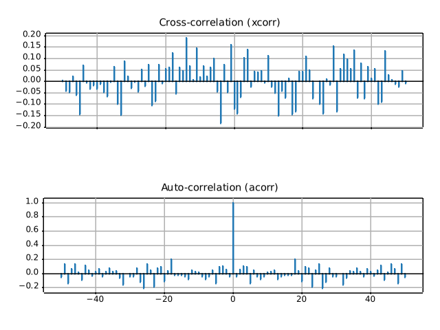
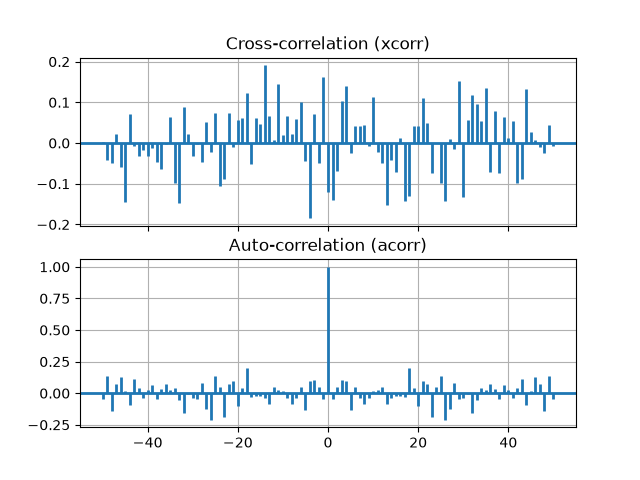
style_sheets/bmh
========================================
Source
"""
========================================
Bayesian Methods for Hackers style sheet
========================================
This example demonstrates the style used in the Bayesian Methods for Hackers
[1]_ online book.
.. [1] http://camdavidsonpilon.github.io/Probabilistic-Programming-and-Bayesian-Methods-for-Hackers/
"""
import matplotlib.pyplot as plt
import numpy as np
# Fixing random state for reproducibility
np.random.seed(19680801)
plt.style.use('bmh')
def plot_beta_hist(ax, a, b):
ax.hist(np.random.beta(a, b, size=10000),
histtype="stepfilled", bins=25, alpha=0.8, density=True)
fig, ax = plt.subplots()
plot_beta_hist(ax, 10, 10)
plot_beta_hist(ax, 4, 12)
plot_beta_hist(ax, 50, 12)
plot_beta_hist(ax, 6, 55)
ax.set_title("'bmh' style sheet")
plt.show()
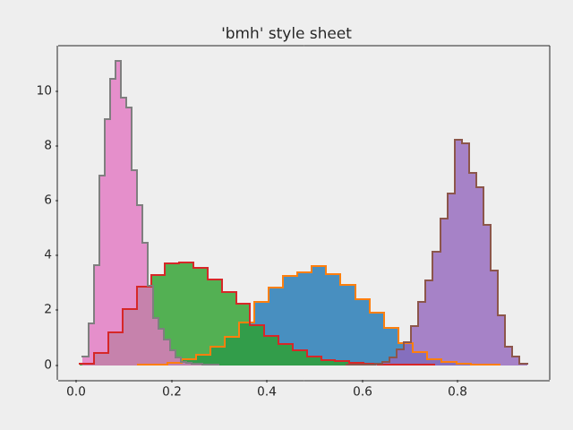
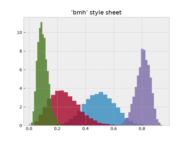
style_sheets/dark_background
===========================
Source
"""
===========================
Dark background style sheet
===========================
This example demonstrates the "dark_background" style, which uses white for
elements that are typically black (text, borders, etc). Note that not all plot
elements default to colors defined by an rc parameter.
"""
import matplotlib.pyplot as plt
import numpy as np
plt.style.use('dark_background')
fig, ax = plt.subplots()
L = 6
x = np.linspace(0, L)
ncolors = len(plt.rcParams['axes.prop_cycle'])
shift = np.linspace(0, L, ncolors, endpoint=False)
for s in shift:
ax.plot(x, np.sin(x + s), 'o-')
ax.set_xlabel('x-axis')
ax.set_ylabel('y-axis')
ax.set_title("'dark_background' style sheet")
plt.show()
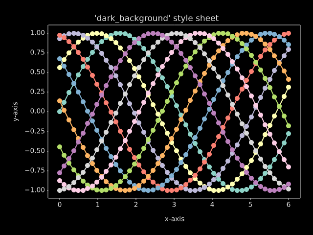
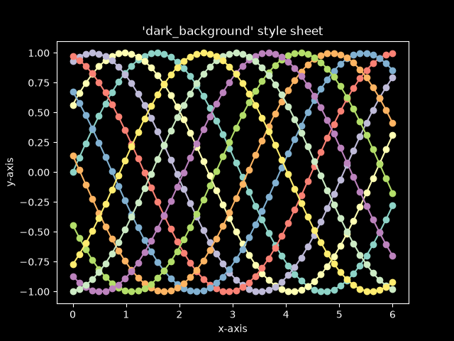
style_sheets/fivethirtyeight
===========================
Source
"""
===========================
FiveThirtyEight style sheet
===========================
This shows an example of the "fivethirtyeight" styling, which
tries to replicate the styles from FiveThirtyEight.com.
"""
import matplotlib.pyplot as plt
import numpy as np
plt.style.use('fivethirtyeight')
x = np.linspace(0, 10)
# Fixing random state for reproducibility
np.random.seed(19680801)
fig, ax = plt.subplots()
ax.plot(x, np.sin(x) + x + np.random.randn(50))
ax.plot(x, np.sin(x) + 0.5 * x + np.random.randn(50))
ax.plot(x, np.sin(x) + 2 * x + np.random.randn(50))
ax.plot(x, np.sin(x) - 0.5 * x + np.random.randn(50))
ax.plot(x, np.sin(x) - 2 * x + np.random.randn(50))
ax.plot(x, np.sin(x) + np.random.randn(50))
ax.set_title("'fivethirtyeight' style sheet")
plt.show()
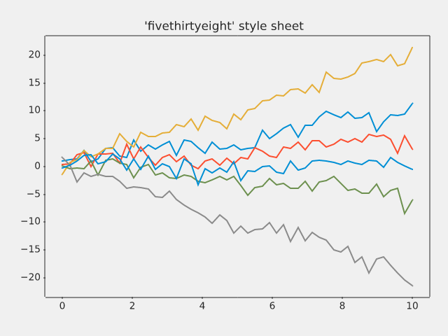
style_sheets/ggplot
==================
Source
"""
==================
ggplot style sheet
==================
This example demonstrates the "ggplot" style, which adjusts the style to
emulate ggplot_ (a popular plotting package for R_).
These settings were shamelessly stolen from [1]_ (with permission).
.. [1] https://everyhue.me/posts/sane-color-scheme-for-matplotlib/
.. _ggplot: https://ggplot2.tidyverse.org/
.. _R: https://www.r-project.org/
"""
import matplotlib.pyplot as plt
import numpy as np
plt.style.use('ggplot')
# Fixing random state for reproducibility
np.random.seed(19680801)
fig, axs = plt.subplots(ncols=2, nrows=2)
ax1, ax2, ax3, ax4 = axs.flat
# scatter plot (Note: `plt.scatter` doesn't use default colors)
x, y = np.random.normal(size=(2, 200))
ax1.plot(x, y, 'o')
# sinusoidal lines with colors from default color cycle
L = 2*np.pi
x = np.linspace(0, L)
ncolors = len(plt.rcParams['axes.prop_cycle'])
shift = np.linspace(0, L, ncolors, endpoint=False)
for s in shift:
ax2.plot(x, np.sin(x + s), '-')
ax2.margins(0)
# bar graphs
x = np.arange(5)
y1, y2 = np.random.randint(1, 25, size=(2, 5))
width = 0.25
ax3.bar(x, y1, width)
ax3.bar(x + width, y2, width,
color=list(plt.rcParams['axes.prop_cycle'])[2]['color'])
ax3.set_xticks(x + width, labels=['a', 'b', 'c', 'd', 'e'])
# circles with colors from default color cycle
for i, color in enumerate(plt.rcParams['axes.prop_cycle']):
xy = np.random.normal(size=2)
ax4.add_patch(plt.Circle(xy, radius=0.3, color=color['color']))
ax4.axis('equal')
ax4.margins(0)
plt.show()
style_sheets/grayscale
=====================
Source
"""
=====================
Grayscale style sheet
=====================
This example demonstrates the "grayscale" style sheet, which changes all colors
that are defined as `.rcParams` to grayscale. Note, however, that not all
plot elements respect `.rcParams`.
"""
import matplotlib.pyplot as plt
import numpy as np
# Fixing random state for reproducibility
np.random.seed(19680801)
def color_cycle_example(ax):
L = 6
x = np.linspace(0, L)
ncolors = len(plt.rcParams['axes.prop_cycle'])
shift = np.linspace(0, L, ncolors, endpoint=False)
for s in shift:
ax.plot(x, np.sin(x + s), 'o-')
def image_and_patch_example(ax):
ax.imshow(np.random.random(size=(20, 20)), interpolation='none')
c = plt.Circle((5, 5), radius=5, label='patch')
ax.add_patch(c)
plt.style.use('grayscale')
fig, (ax1, ax2) = plt.subplots(ncols=2)
fig.suptitle("'grayscale' style sheet")
color_cycle_example(ax1)
image_and_patch_example(ax2)
plt.show()
style_sheets/petroff10
====================
Source
"""
====================
Petroff style sheets
====================
This example demonstrates the "petroffN" styles, which implement the 6-, 8- and
10-color sequences developed by Matthew A. Petroff [1]_ for accessible data
visualization. The styles balance aesthetics with accessibility considerations,
making them suitable for various types of plots while ensuring readability and
distinction between data series.
.. [1] https://arxiv.org/abs/2107.02270
"""
import matplotlib.pyplot as plt
import numpy as np
def colored_lines_example(ax):
t = np.linspace(-10, 10, 100)
nb_colors = len(plt.rcParams['axes.prop_cycle'])
shifts = np.linspace(-5, 5, nb_colors)
amplitudes = np.linspace(1, 1.5, nb_colors)
for t0, a in zip(shifts, amplitudes):
y = a / (1 + np.exp(-(t - t0)))
line, = ax.plot(t, y, '-')
point_indices = np.linspace(0, len(t) - 1, 20, dtype=int)
ax.plot(t[point_indices], y[point_indices], 'o', color=line.get_color())
ax.set_xlim(-10, 10)
def image_and_patch_example(ax):
ax.imshow(np.random.random(size=(20, 20)), interpolation='none')
c = plt.Circle((5, 5), radius=5, label='patch')
ax.add_patch(c)
fig = plt.figure(figsize=(6.4, 9.6), layout='compressed')
sfigs = fig.subfigures(nrows=3)
for style, sfig in zip(['petroff6', 'petroff8', 'petroff10'], sfigs):
sfig.suptitle(f"'{style}' style sheet")
with plt.style.context(style):
ax1, ax2 = sfig.subplots(ncols=2)
colored_lines_example(ax1)
image_and_patch_example(ax2)
plt.show()
style_sheets/plot_solarizedlight2
==========================
Source
"""
==========================
Solarized Light stylesheet
==========================
This shows an example of "Solarized_Light" styling, which
tries to replicate the styles of:
- https://ethanschoonover.com/solarized/
- https://github.com/jrnold/ggthemes
- http://www.pygal.org/en/stable/documentation/builtin_styles.html#light-solarized
and work of:
- https://github.com/tonysyu/mpltools
using all 8 accents of the color palette - starting with blue
Still TODO:
- Create alpha values for bar and stacked charts. .33 or .5
- Apply Layout Rules
"""
import matplotlib.pyplot as plt
import numpy as np
# Fixing random state for reproducibility
np.random.seed(19680801)
x = np.linspace(0, 10)
with plt.style.context('Solarize_Light2'):
plt.plot(x, np.sin(x) + x + np.random.randn(50))
plt.plot(x, np.sin(x) + 2 * x + np.random.randn(50))
plt.plot(x, np.sin(x) + 3 * x + np.random.randn(50))
plt.plot(x, np.sin(x) + 4 * x + np.random.randn(50))
plt.plot(x, np.sin(x) + 5 * x + np.random.randn(50))
plt.plot(x, np.sin(x) + 6 * x + np.random.randn(50))
plt.plot(x, np.sin(x) + 7 * x + np.random.randn(50))
plt.plot(x, np.sin(x) + 8 * x + np.random.randn(50))
# Number of accent colors in the color scheme
plt.title('8 Random Lines - Line')
plt.xlabel('x label', fontsize=14)
plt.ylabel('y label', fontsize=14)
plt.show()
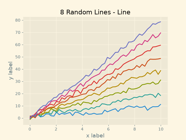
style_sheets/style_sheets_reference
======================
Source
"""
======================
Style sheets reference
======================
This script demonstrates the different available style sheets on a
common set of example plots: scatter plot, image, bar graph, patches,
line plot and histogram.
Any of these style sheets can be imported (i.e. activated) by its name.
For example for the ggplot style:
>>> plt.style.use('ggplot')
The names of the available style sheets can be found
in the list `matplotlib.style.available`
(they are also printed in the corner of each plot below).
See more details in :ref:`Customizing Matplotlib
using style sheets<customizing-with-style-sheets>`.
"""
import matplotlib.pyplot as plt
import numpy as np
import matplotlib.colors as mcolors
from matplotlib.patches import Rectangle
# Fixing random state for reproducibility
np.random.seed(19680801)
def plot_scatter(ax, prng, nb_samples=100):
"""Scatter plot."""
for mu, sigma, marker in [(-.5, 0.75, 'o'), (0.75, 1., 's')]:
x, y = prng.normal(loc=mu, scale=sigma, size=(2, nb_samples))
ax.plot(x, y, ls='none', marker=marker)
ax.set_xlabel('X-label')
ax.set_title('Axes title')
return ax
def plot_colored_lines(ax):
"""Plot lines with colors following the style color cycle."""
t = np.linspace(-10, 10, 100)
def sigmoid(t, t0):
return 1 / (1 + np.exp(-(t - t0)))
nb_colors = len(plt.rcParams['axes.prop_cycle'])
shifts = np.linspace(-5, 5, nb_colors)
amplitudes = np.linspace(1, 1.5, nb_colors)
for t0, a in zip(shifts, amplitudes):
ax.plot(t, a * sigmoid(t, t0), '-')
ax.set_xlim(-10, 10)
return ax
def plot_bar_graphs(ax, prng, min_value=5, max_value=25, nb_samples=5):
"""Plot two bar graphs side by side, with letters as x-tick labels."""
x = np.arange(nb_samples)
ya, yb = prng.randint(min_value, max_value, size=(2, nb_samples))
width = 0.25
ax.bar(x, ya, width)
ax.bar(x + width, yb, width, color='C2')
ax.set_xticks(x + width, labels=['a', 'b', 'c', 'd', 'e'])
return ax
def plot_colored_circles(ax, prng, nb_samples=15):
"""
Plot circle patches.
NB: draws a fixed amount of samples, rather than using the length of
the color cycle, because different styles may have different numbers
of colors.
"""
for sty_dict, j in zip(plt.rcParams['axes.prop_cycle'](),
range(nb_samples)):
ax.add_patch(plt.Circle(prng.normal(scale=3, size=2),
radius=1.0, color=sty_dict['color']))
ax.grid(visible=True)
# Add title for enabling grid
plt.title('ax.grid(True)', family='monospace', fontsize='small')
ax.set_xlim([-4, 8])
ax.set_ylim([-5, 6])
ax.set_aspect('equal', adjustable='box') # to plot circles as circles
return ax
def plot_image_and_patch(ax, prng, size=(20, 20)):
"""Plot an image with random values and superimpose a circular patch."""
values = prng.random_sample(size=size)
ax.imshow(values, interpolation='none')
c = plt.Circle((5, 5), radius=5, label='patch')
ax.add_patch(c)
# Remove ticks
ax.set_xticks([])
ax.set_yticks([])
def plot_histograms(ax, prng, nb_samples=10000):
"""Plot 4 histograms and a text annotation."""
params = ((10, 10), (4, 12), (50, 12), (6, 55))
for a, b in params:
values = prng.beta(a, b, size=nb_samples)
ax.hist(values, histtype="stepfilled", bins=30,
alpha=0.8, density=True)
# Add a small annotation.
ax.annotate('Annotation', xy=(0.25, 4.25),
xytext=(0.9, 0.9), textcoords=ax.transAxes,
va="top", ha="right",
bbox=dict(boxstyle="round", alpha=0.2),
arrowprops=dict(
arrowstyle="->",
connectionstyle="angle,angleA=-95,angleB=35,rad=10"),
)
return ax
def plot_figure(style_label=""):
"""Setup and plot the demonstration figure with a given style."""
# Use a dedicated RandomState instance to draw the same "random" values
# across the different figures.
prng = np.random.RandomState(96917002)
fig, axs = plt.subplots(ncols=6, nrows=1, num=style_label,
figsize=(14.8, 2.8), layout='constrained')
# make a suptitle, in the same style for all subfigures,
# except those with dark backgrounds, which get a lighter color:
background_color = mcolors.rgb_to_hsv(
mcolors.to_rgb(plt.rcParams['figure.facecolor']))[2]
if background_color < 0.5:
title_color = [0.8, 0.8, 1]
else:
title_color = np.array([19, 6, 84]) / 256
fig.suptitle(style_label, x=0.01, ha='left', color=title_color,
fontsize=14, fontfamily='DejaVu Sans', fontweight='normal')
plot_scatter(axs[0], prng)
plot_image_and_patch(axs[1], prng)
plot_bar_graphs(axs[2], prng)
plot_colored_lines(axs[3])
plot_histograms(axs[4], prng)
plot_colored_circles(axs[5], prng)
# add divider
rec = Rectangle((1 + 0.025, -2), 0.05, 16,
clip_on=False, color='gray')
axs[4].add_artist(rec)
if __name__ == "__main__":
# Set up a list of all available styles, in alphabetical order but
# the `default` and `classic` ones, which will be forced resp. in
# first and second position.
# styles with leading underscores are for internal use such as testing
# and plot types gallery. These are excluded here.
style_list = ['default', 'classic'] + sorted(
style for style in plt.style.available
if style != 'classic' and not style.startswith('_'))
# Plot a demonstration figure for every available style sheet.
for style_label in style_list:
with plt.rc_context({"figure.max_open_warning": len(style_list)}):
with plt.style.context(style_label):
plot_figure(style_label=style_label)
plt.show()


subplots_axes_and_figures/align_labels_demo
=======================
Source
"""
=======================
Align labels and titles
=======================
Aligning xlabel, ylabel, and title using `.Figure.align_xlabels`,
`.Figure.align_ylabels`, and `.Figure.align_titles`.
`.Figure.align_labels` wraps the x and y label functions.
We align the xlabels and ylabels using short calls to `.Figure.align_xlabels`
and `.Figure.align_ylabels`. We also show a manual way to align the ylabels
using the `~.Axis.set_label_coords` method of the yaxis object. Note this requires
knowing a good offset value which is hardcoded.
.. redirect-from:: /gallery/pyplots/align_ylabels
"""
import matplotlib.pyplot as plt
import numpy as np
fig, axs = plt.subplots(2, 3, figsize=(8.9, 5.5),
layout='constrained', gridspec_kw={'wspace': 0.1})
# add sample data and labels
for ax in axs.flat:
scale = 2000 if ax.get_subplotspec().is_first_row() else 1
ax.plot(scale * (1 - np.exp(-np.linspace(0, 5, 100))))
if ax.get_subplotspec().is_last_row():
ax.set_xlabel('xlabel', bbox=dict(facecolor='yellow', pad=5, alpha=0.2))
ax.set_ylabel('ylabel', bbox=dict(facecolor='yellow', pad=5, alpha=0.2))
ax.set_ylim(0, scale)
# Modify ticks to get different margins in some plots
axs[0, 0].xaxis.tick_top()
axs[1, 2].tick_params(axis='x', rotation=55)
axs[0, 0].set_title('ylabels not aligned')
# Align labels
fig.align_titles() # Align titles
fig.align_xlabels() # Align all x-axis labels
fig.align_ylabels(axs[:, 1]) # Align only the second column's y-labels
axs[0, 1].set_title('fig.align_ylabels()')
# Manually adjust y-labels for the third column
for ax in axs[:, 2]:
ax.yaxis.set_label_coords(-0.3, 0.5)
axs[0, 2].set_title('ylabels manually aligned')
plt.show()
# %%
#
# .. admonition:: References
#
# The use of the following functions, methods, classes and modules is shown
# in this example:
#
# - `matplotlib.figure.Figure.align_xlabels`
# - `matplotlib.figure.Figure.align_ylabels`
# - `matplotlib.figure.Figure.align_labels`
# - `matplotlib.figure.Figure.align_titles`
# - `matplotlib.axis.Axis.set_label_coords`
# - `matplotlib.axes.Axes.plot` / `matplotlib.pyplot.plot`
# - `matplotlib.axes.Axes.set_title`
# - `matplotlib.axes.Axes.set_ylabel`
# - `matplotlib.axes.Axes.set_ylim`
# %%
# .. tags::
#
# component: label
# component: title
# styling: position
# level: beginner
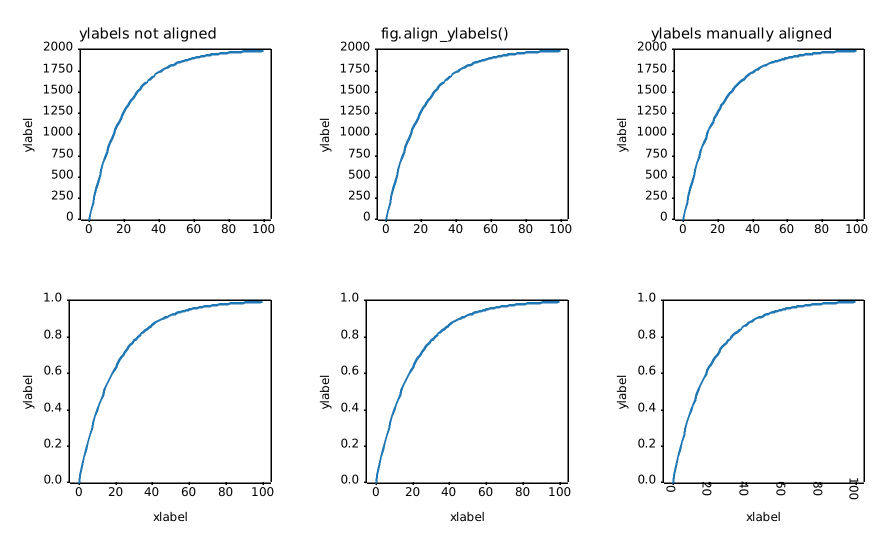
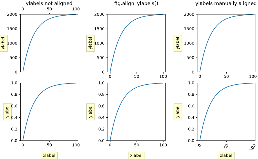
subplots_axes_and_figures/auto_subplots_adjust
===========================================
Source
"""
===========================================
Programmatically control subplot adjustment
===========================================
.. note::
This example is primarily intended to show some advanced concepts in
Matplotlib.
If you are only looking for having enough space for your labels, it is
almost always simpler and good enough to either set the subplot parameters
manually using `.Figure.subplots_adjust`, or use one of the automatic
layout mechanisms
(:ref:`constrainedlayout_guide` or
:ref:`tight_layout_guide`).
This example describes a user-defined way to read out Artist sizes and
set the subplot parameters accordingly. Its main purpose is to illustrate
some advanced concepts like reading out text positions, working with
bounding boxes and transforms and using
:ref:`events <event-handling>`. But it can also serve as a starting
point if you want to automate the layouting and need more flexibility than
tight layout and constrained layout.
Below, we collect the bounding boxes of all y-labels and move the left border
of the subplot to the right so that it leaves enough room for the union of all
the bounding boxes.
There's one catch with calculating text bounding boxes:
Querying the text bounding boxes (`.Text.get_window_extent`) needs a
renderer (`.RendererBase` instance), to calculate the text size. This renderer
is only available after the figure has been drawn (`.Figure.draw`).
A solution to this is putting the adjustment logic in a draw callback.
This function is executed after the figure has been drawn. It can now check
if the subplot leaves enough room for the text. If not, the subplot parameters
are updated and second draw is triggered.
.. redirect-from:: /gallery/pyplots/auto_subplots_adjust
"""
import matplotlib.pyplot as plt
import matplotlib.transforms as mtransforms
fig, ax = plt.subplots()
ax.plot(range(10))
ax.set_yticks([2, 5, 7], labels=['really, really, really', 'long', 'labels'])
def on_draw(event):
bboxes = []
for label in ax.get_yticklabels():
# Bounding box in pixels
bbox_px = label.get_window_extent()
# Transform to relative figure coordinates. This is the inverse of
# transFigure.
bbox_fig = bbox_px.transformed(fig.transFigure.inverted())
bboxes.append(bbox_fig)
# the bbox that bounds all the bboxes, again in relative figure coords
bbox = mtransforms.Bbox.union(bboxes)
if fig.subplotpars.left < bbox.width:
# Move the subplot left edge more to the right
fig.subplots_adjust(left=1.1*bbox.width) # pad a little
fig.canvas.draw()
fig.canvas.mpl_connect('draw_event', on_draw)
plt.show()
# %%
#
# .. admonition:: References
#
# The use of the following functions, methods, classes and modules is shown
# in this example:
#
# - `matplotlib.artist.Artist.get_window_extent`
# - `matplotlib.transforms.Bbox`
# - `matplotlib.transforms.BboxBase.transformed`
# - `matplotlib.transforms.BboxBase.union`
# - `matplotlib.transforms.Transform.inverted`
# - `matplotlib.figure.Figure.subplots_adjust`
# - `matplotlib.gridspec.SubplotParams`
# - `matplotlib.backend_bases.FigureCanvasBase.mpl_connect`
#
# .. tags::
#
# component: subplot
# plot-type: line
# styling: position
# level: advanced
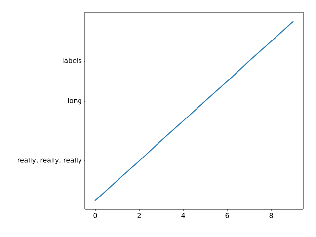
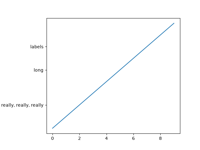
subplots_axes_and_figures/axes_box_aspect
===============
Source
"""
===============
Axes box aspect
===============
This demo shows how to set the aspect of an Axes box directly via
`~.Axes.set_box_aspect`. The box aspect is the ratio between Axes height
and Axes width in physical units, independent of the data limits.
This is useful to e.g. produce a square plot, independent of the data it
contains, or to have a usual plot with the same axes dimensions next to
an image plot with fixed (data-)aspect.
The following lists a few use cases for `~.Axes.set_box_aspect`.
"""
# %%
# A square Axes, independent of data
# ----------------------------------
#
# Produce a square Axes, no matter what the data limits are.
import matplotlib.pyplot as plt
import numpy as np
fig1, ax = plt.subplots()
ax.set_xlim(300, 400)
ax.set_box_aspect(1)
plt.show()
# %%
# Shared square Axes
# ------------------
#
# Produce shared subplots that are squared in size.
#
fig2, (ax, ax2) = plt.subplots(ncols=2, sharey=True)
ax.plot([1, 5], [0, 10])
ax2.plot([100, 500], [10, 15])
ax.set_box_aspect(1)
ax2.set_box_aspect(1)
plt.show()
# %%
# Square twin Axes
# ----------------
#
# Produce a square Axes, with a twin Axes. The twinned Axes takes over the
# box aspect of the parent.
#
fig3, ax = plt.subplots()
ax2 = ax.twinx()
ax.plot([0, 10])
ax2.plot([12, 10])
ax.set_box_aspect(1)
plt.show()
# %%
# Normal plot next to image
# -------------------------
#
# When creating an image plot with fixed data aspect and the default
# ``adjustable="box"`` next to a normal plot, the Axes would be unequal in
# height. `~.Axes.set_box_aspect` provides an easy solution to that by allowing
# to have the normal plot's Axes use the images dimensions as box aspect.
#
# This example also shows that *constrained layout* interplays nicely with
# a fixed box aspect.
fig4, (ax, ax2) = plt.subplots(ncols=2, layout="constrained")
np.random.seed(19680801) # Fixing random state for reproducibility
im = np.random.rand(16, 27)
ax.imshow(im)
ax2.plot([23, 45])
ax2.set_box_aspect(im.shape[0]/im.shape[1])
plt.show()
# %%
# Square joint/marginal plot
# --------------------------
#
# It may be desirable to show marginal distributions next to a plot of joint
# data. The following creates a square plot with the box aspect of the
# marginal Axes being equal to the width- and height-ratios of the gridspec.
# This ensures that all Axes align perfectly, independent on the size of the
# figure.
fig5, axs = plt.subplots(2, 2, sharex="col", sharey="row",
gridspec_kw=dict(height_ratios=[1, 3],
width_ratios=[3, 1]))
axs[0, 1].set_visible(False)
axs[0, 0].set_box_aspect(1/3)
axs[1, 0].set_box_aspect(1)
axs[1, 1].set_box_aspect(3/1)
np.random.seed(19680801) # Fixing random state for reproducibility
x, y = np.random.randn(2, 400) * [[.5], [180]]
axs[1, 0].scatter(x, y)
axs[0, 0].hist(x)
axs[1, 1].hist(y, orientation="horizontal")
plt.show()
# %%
# Set data aspect with box aspect
# -------------------------------
#
# When setting the box aspect, one may still set the data aspect as well.
# Here we create an Axes with a box twice as long as it is tall and use
# an "equal" data aspect for its contents, i.e. the circle actually
# stays circular.
fig6, ax = plt.subplots()
ax.add_patch(plt.Circle((5, 3), 1))
ax.set_aspect("equal", adjustable="datalim")
ax.set_box_aspect(0.5)
ax.autoscale()
plt.show()
# %%
# Box aspect for many subplots
# ----------------------------
#
# It is possible to pass the box aspect to an Axes at initialization. The
# following creates a 2 by 3 subplot grid with all square Axes.
fig7, axs = plt.subplots(2, 3, subplot_kw=dict(box_aspect=1),
sharex=True, sharey=True, layout="constrained")
for i, ax in enumerate(axs.flat):
ax.scatter(i % 3, -((i // 3) - 0.5)*200, c=[plt.colormaps["hsv"](i / 6)], s=300)
plt.show()
# %%
#
# .. admonition:: References
#
# The use of the following functions, methods, classes and modules is shown
# in this example:
#
# - `matplotlib.axes.Axes.set_box_aspect`
#
# .. tags::
#
# component: axes
# styling: size
# level: beginner
subplots_axes_and_figures/axes_demo
=========
Source
"""
=========
Axes Demo
=========
Example use of ``fig.add_axes`` to create inset Axes within the main plot Axes.
Please see also the :ref:`axes_grid_examples` section, and the following three
examples:
- :doc:`/gallery/subplots_axes_and_figures/zoom_inset_axes`
- :doc:`/gallery/axes_grid1/inset_locator_demo`
- :doc:`/gallery/axes_grid1/inset_locator_demo2`
"""
import matplotlib.pyplot as plt
import numpy as np
np.random.seed(19680801) # Fixing random state for reproducibility.
# create some data to use for the plot
dt = 0.001
t = np.arange(0.0, 10.0, dt)
r = np.exp(-t[:1000] / 0.05) # impulse response
x = np.random.randn(len(t))
s = np.convolve(x, r)[:len(x)] * dt # colored noise
fig, main_ax = plt.subplots()
main_ax.plot(t, s)
main_ax.set_xlim(0, 1)
main_ax.set_ylim(1.1 * np.min(s), 2 * np.max(s))
main_ax.set_xlabel('time (s)')
main_ax.set_ylabel('current (nA)')
main_ax.set_title('Gaussian colored noise')
# this is an inset Axes over the main Axes
right_inset_ax = fig.add_axes((.65, .6, .2, .2), facecolor='k')
right_inset_ax.hist(s, 400, density=True)
right_inset_ax.set(title='Probability', xticks=[], yticks=[])
# this is another inset Axes over the main Axes
left_inset_ax = fig.add_axes((.2, .6, .2, .2), facecolor='k')
left_inset_ax.plot(t[:len(r)], r)
left_inset_ax.set(title='Impulse response', xlim=(0, .2), xticks=[], yticks=[])
plt.show()
# %%
# .. tags::
#
# component: axes
# plot-type: line
# plot-type: histogram
# level: beginner
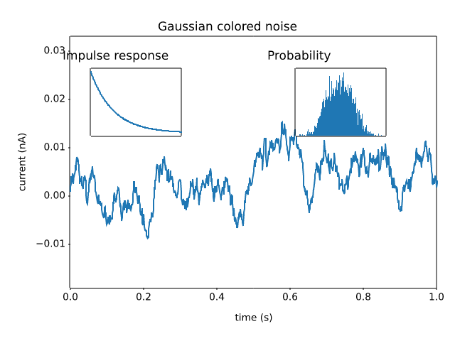
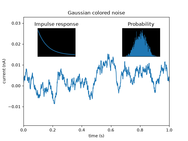
subplots_axes_and_figures/axes_margins
======================================================
Source
"""
======================================================
Controlling view limits using margins and sticky_edges
======================================================
The first figure in this example shows how to zoom in and out of a
plot using `~.Axes.margins` instead of `~.Axes.set_xlim` and
`~.Axes.set_ylim`. The second figure demonstrates the concept of
edge "stickiness" introduced by certain methods and artists and how
to effectively work around that.
"""
import matplotlib.pyplot as plt
import numpy as np
from matplotlib.patches import Polygon
def f(t):
return np.exp(-t) * np.cos(2*np.pi*t)
t1 = np.arange(0.0, 3.0, 0.01)
ax1 = plt.subplot(212)
ax1.margins(0.05) # Default margin is 0.05, value 0 means fit
ax1.plot(t1, f(t1))
ax2 = plt.subplot(221)
ax2.margins(2, 2) # Values >0.0 zoom out
ax2.plot(t1, f(t1))
ax2.set_title('Zoomed out')
ax3 = plt.subplot(222)
ax3.margins(x=0, y=-0.25) # Values in (-0.5, 0.0) zooms in to center
ax3.plot(t1, f(t1))
ax3.set_title('Zoomed in')
plt.show()
# %%
#
# On the "stickiness" of certain plotting methods
# """""""""""""""""""""""""""""""""""""""""""""""
#
# Some plotting functions make the axis limits "sticky" or immune to the will
# of the `~.Axes.margins` methods. For instance, `~.Axes.imshow` and
# `~.Axes.pcolor` expect the user to want the limits to be tight around the
# pixels shown in the plot. If this behavior is not desired, you need to set
# `~.Axes.use_sticky_edges` to `False`. Consider the following example:
y, x = np.mgrid[:5, 1:6]
poly_coords = [
(0.25, 2.75), (3.25, 2.75),
(2.25, 0.75), (0.25, 0.75)
]
fig, (ax1, ax2) = plt.subplots(ncols=2)
# Here we set the stickiness of the Axes object...
# ax1 we'll leave as the default, which uses sticky edges
# and we'll turn off stickiness for ax2
ax2.use_sticky_edges = False
for ax, status in zip((ax1, ax2), ('Is', 'Is Not')):
cells = ax.pcolor(x, y, x+y, cmap='inferno', shading='auto') # sticky
ax.add_patch(
Polygon(poly_coords, color='forestgreen', alpha=0.5)
) # not sticky
ax.margins(x=0.1, y=0.05)
ax.set_aspect('equal')
ax.set_title(f'{status} Sticky')
plt.show()
# %%
#
# .. admonition:: References
#
# The use of the following functions, methods, classes and modules is shown
# in this example:
#
# - `matplotlib.axes.Axes.margins` / `matplotlib.pyplot.margins`
# - `matplotlib.axes.Axes.use_sticky_edges`
# - `matplotlib.axes.Axes.pcolor` / `matplotlib.pyplot.pcolor`
# - `matplotlib.patches.Polygon`
#
# .. tags::
#
# component: axes
# plot-type: line
# plot-type: imshow
# plot-type: pcolor
# level: beginner
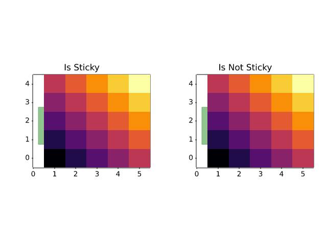
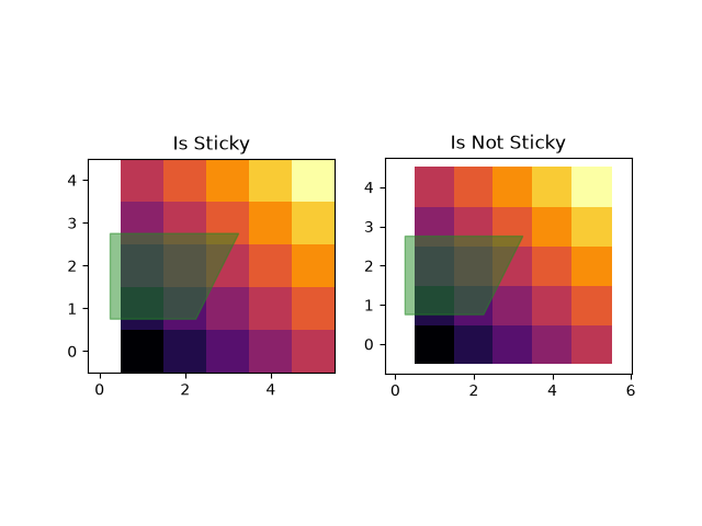
subplots_axes_and_figures/axes_props
===============
Source
""" =============== Axes properties =============== You can control the axis tick and grid properties """ import matplotlib.pyplot as plt import numpy as np t = np.arange(0.0, 2.0, 0.01) s = np.sin(2 * np.pi * t) fig, ax = plt.subplots() ax.plot(t, s) ax.grid(True, linestyle='-.') ax.tick_params(labelcolor='r', labelsize='medium', width=3) plt.show() # %% # .. tags:: # # component: ticks # plot-type: line # level: beginner
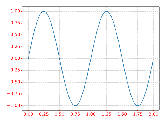
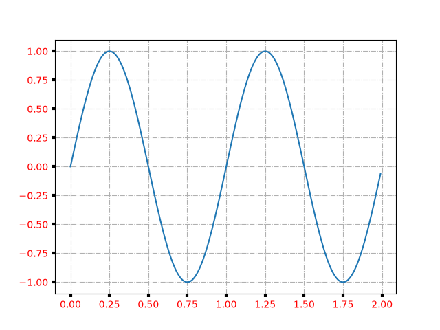
subplots_axes_and_figures/axes_zoom_effect
================
Source
"""
================
Axes zoom effect
================
"""
import matplotlib.pyplot as plt
from matplotlib.transforms import Bbox, TransformedBbox, blended_transform_factory
from mpl_toolkits.axes_grid1.inset_locator import (BboxConnector, BboxConnectorPatch,
BboxPatch)
def connect_bbox(bbox1, bbox2,
loc1a, loc2a, loc1b, loc2b,
prop_lines, prop_patches=None):
if prop_patches is None:
prop_patches = {
**prop_lines,
"alpha": prop_lines.get("alpha", 1) * 0.2,
"clip_on": False,
}
c1 = BboxConnector(
bbox1, bbox2, loc1=loc1a, loc2=loc2a, clip_on=False, **prop_lines)
c2 = BboxConnector(
bbox1, bbox2, loc1=loc1b, loc2=loc2b, clip_on=False, **prop_lines)
bbox_patch1 = BboxPatch(bbox1, **prop_patches)
bbox_patch2 = BboxPatch(bbox2, **prop_patches)
p = BboxConnectorPatch(bbox1, bbox2,
loc1a=loc1a, loc2a=loc2a, loc1b=loc1b, loc2b=loc2b,
clip_on=False,
**prop_patches)
return c1, c2, bbox_patch1, bbox_patch2, p
def zoom_effect01(ax1, ax2, xmin, xmax, **kwargs):
"""
Connect *ax1* and *ax2*. The *xmin*-to-*xmax* range in both Axes will
be marked.
Parameters
----------
ax1
The main Axes.
ax2
The zoomed Axes.
xmin, xmax
The limits of the colored area in both plot Axes.
**kwargs
Arguments passed to the patch constructor.
"""
bbox = Bbox.from_extents(xmin, 0, xmax, 1)
mybbox1 = TransformedBbox(bbox, ax1.get_xaxis_transform())
mybbox2 = TransformedBbox(bbox, ax2.get_xaxis_transform())
prop_patches = {**kwargs, "ec": "none", "alpha": 0.2}
c1, c2, bbox_patch1, bbox_patch2, p = connect_bbox(
mybbox1, mybbox2,
loc1a=3, loc2a=2, loc1b=4, loc2b=1,
prop_lines=kwargs, prop_patches=prop_patches)
ax1.add_patch(bbox_patch1)
ax2.add_patch(bbox_patch2)
ax2.add_patch(c1)
ax2.add_patch(c2)
ax2.add_patch(p)
return c1, c2, bbox_patch1, bbox_patch2, p
def zoom_effect02(ax1, ax2, **kwargs):
"""
ax1 : the main Axes
ax1 : the zoomed Axes
Similar to zoom_effect01. The xmin & xmax will be taken from the
ax1.viewLim.
"""
tt = ax1.transScale + (ax1.transLimits + ax2.transAxes)
trans = blended_transform_factory(ax2.transData, tt)
mybbox1 = ax1.bbox
mybbox2 = TransformedBbox(ax1.viewLim, trans)
prop_patches = {**kwargs, "ec": "none", "alpha": 0.2}
c1, c2, bbox_patch1, bbox_patch2, p = connect_bbox(
mybbox1, mybbox2,
loc1a=3, loc2a=2, loc1b=4, loc2b=1,
prop_lines=kwargs, prop_patches=prop_patches)
ax1.add_patch(bbox_patch1)
ax2.add_patch(bbox_patch2)
ax2.add_patch(c1)
ax2.add_patch(c2)
ax2.add_patch(p)
return c1, c2, bbox_patch1, bbox_patch2, p
axs = plt.figure().subplot_mosaic([
["zoom1", "zoom2"],
["main", "main"],
])
axs["main"].set(xlim=(0, 5))
zoom_effect01(axs["zoom1"], axs["main"], 0.2, 0.8)
axs["zoom2"].set(xlim=(2, 3))
zoom_effect02(axs["zoom2"], axs["main"])
plt.show()
# %%
# .. tags::
#
# component: subplot
# component: transform
# level: advanced
ImportError: cannot import name 'BboxConnector' from 'matplotvite.mpl_toolkits.axes_grid1.inset_locator' (/home/runner/work/matplotvite/matplotvite/python/matplotvite/mpl_toolkits/axes_grid1/inset_locator.py)
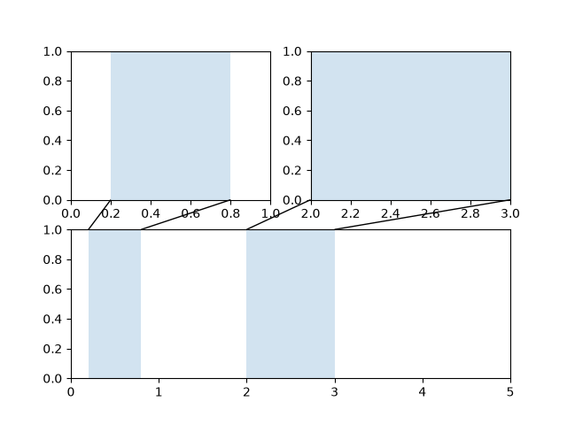
subplots_axes_and_figures/axhspan_demo
==============================
Source
""" ============================== Draw regions that span an Axes ============================== `~.Axes.axhspan` and `~.Axes.axvspan` draw rectangles that span the Axes in either the horizontal or vertical direction and are bounded in the other direction. They are often used to highlight data regions. """ import matplotlib.pyplot as plt import numpy as np fig, (ax1, ax2) = plt.subplots(1, 2, figsize=(7, 3)) np.random.seed(19680801) s = 2.9 * np.convolve(np.random.randn(500), np.ones(30) / 30, mode='valid') ax1.plot(s) ax1.axhspan(-1, 1, alpha=0.1) ax1.set(ylim=(-1.5, 1.5), title="axhspan") mu = 8 sigma = 2 x = np.linspace(0, 16, 401) y = np.exp(-((x-mu)**2)/(2*sigma**2)) ax2.axvspan(mu-2*sigma, mu-sigma, color='0.95') ax2.axvspan(mu-sigma, mu+sigma, color='0.9') ax2.axvspan(mu+sigma, mu+2*sigma, color='0.95') ax2.axvline(mu, color='darkgrey', linestyle='--') ax2.plot(x, y) ax2.set(title="axvspan") plt.show() # %% # # .. admonition:: References # # The use of the following functions, methods, classes and modules is shown # in this example: # # - `matplotlib.axes.Axes.axhspan` / `matplotlib.pyplot.axhspan` # - `matplotlib.axes.Axes.axvspan` / `matplotlib.pyplot.axvspan` # # # .. seealso:: # # `~.Axes.axhline`, `~.Axes.axvline`, `~.Axes.axline` draw infinite lines. # # .. tags:: # # styling: shape # plot-type: line # level: beginner
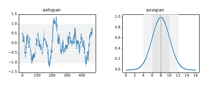
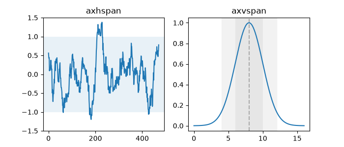
subplots_axes_and_figures/axis_equal_demo
=======================
Source
"""
=======================
Equal axis aspect ratio
=======================
How to set and adjust plots with equal axis aspect ratios.
"""
import matplotlib.pyplot as plt
import numpy as np
# Plot circle of radius 3.
an = np.linspace(0, 2 * np.pi, 100)
fig, axs = plt.subplots(2, 2)
axs[0, 0].plot(3 * np.cos(an), 3 * np.sin(an))
axs[0, 0].set_title('not equal, looks like ellipse', fontsize=10)
axs[0, 1].plot(3 * np.cos(an), 3 * np.sin(an))
axs[0, 1].axis('equal')
axs[0, 1].set_title('equal, looks like circle', fontsize=10)
axs[1, 0].plot(3 * np.cos(an), 3 * np.sin(an))
axs[1, 0].axis('equal')
axs[1, 0].set(xlim=(-3, 3), ylim=(-3, 3))
axs[1, 0].set_title('still a circle, even after changing limits', fontsize=10)
axs[1, 1].plot(3 * np.cos(an), 3 * np.sin(an))
axs[1, 1].set_aspect('equal', 'box')
axs[1, 1].set_title('still a circle, auto-adjusted data limits', fontsize=10)
fig.tight_layout()
plt.show()
# %%
# .. tags::
#
# component: axes
# styling: size
# plot-type: line
# level: beginner
subplots_axes_and_figures/axis_labels_demo
===================
Source
"""
===================
Axis label position
===================
Choose axis label position when calling `~.Axes.set_xlabel` and
`~.Axes.set_ylabel` as well as for colorbar.
"""
import matplotlib.pyplot as plt
fig, ax = plt.subplots()
sc = ax.scatter([1, 2], [1, 2], c=[1, 2])
ax.set_ylabel('YLabel', loc='top')
ax.set_xlabel('XLabel', loc='left')
cbar = fig.colorbar(sc)
cbar.set_label("ZLabel", loc='top')
plt.show()
# %%
# .. tags::
#
# component: axis
# styling: position
# level: beginner
subplots_axes_and_figures/broken_axis
===========
Source
"""
===========
Broken axis
===========
Broken axis example, where the y-axis will have a portion cut out.
"""
import matplotlib.pyplot as plt
import numpy as np
np.random.seed(19680801)
pts = np.random.rand(30)*.2
# Now let's make two outlier points which are far away from everything.
pts[[3, 14]] += .8
# If we were to simply plot pts, we'd lose most of the interesting
# details due to the outliers. So let's 'break' or 'cut-out' the y-axis
# into two portions - use the top (ax1) for the outliers, and the bottom
# (ax2) for the details of the majority of our data
fig, (ax1, ax2) = plt.subplots(2, 1, sharex=True)
fig.subplots_adjust(hspace=0.05) # adjust space between Axes
# plot the same data on both Axes
ax1.plot(pts)
ax2.plot(pts)
# zoom-in / limit the view to different portions of the data
ax1.set_ylim(.78, 1.) # outliers only
ax2.set_ylim(0, .22) # most of the data
# hide the spines between ax and ax2
ax1.spines.bottom.set_visible(False)
ax2.spines.top.set_visible(False)
ax1.xaxis.tick_top()
ax1.tick_params(labeltop=False) # don't put tick labels at the top
ax2.xaxis.tick_bottom()
# Now, let's turn towards the cut-out slanted lines.
# We create line objects in axes coordinates, in which (0,0), (0,1),
# (1,0), and (1,1) are the four corners of the Axes.
# The slanted lines themselves are markers at those locations, such that the
# lines keep their angle and position, independent of the Axes size or scale
# Finally, we need to disable clipping.
d = .5 # proportion of vertical to horizontal extent of the slanted line
kwargs = dict(marker=[(-1, -d), (1, d)], markersize=12,
linestyle="none", color='k', mec='k', mew=1, clip_on=False)
ax1.plot([0, 1], [0, 0], transform=ax1.transAxes, **kwargs)
ax2.plot([0, 1], [1, 1], transform=ax2.transAxes, **kwargs)
plt.show()
# %%
# .. tags::
#
# component: axis
# plot-type: line
# level: intermediate
subplots_axes_and_figures/custom_figure_class
========================
Source
"""
========================
Custom Figure subclasses
========================
You can pass a `.Figure` subclass to `.pyplot.figure` if you want to change
the default behavior of the figure.
This example defines a `.Figure` subclass ``WatermarkFigure`` that accepts an
additional parameter ``watermark`` to display a custom watermark text. The
figure is created using the ``FigureClass`` parameter of `.pyplot.figure`.
The additional ``watermark`` parameter is passed on to the subclass
constructor.
"""
import matplotlib.pyplot as plt
import numpy as np
from matplotlib.figure import Figure
class WatermarkFigure(Figure):
"""A figure with a text watermark."""
def __init__(self, *args, watermark=None, **kwargs):
super().__init__(*args, **kwargs)
if watermark is not None:
bbox = dict(boxstyle='square', lw=3, ec='gray',
fc=(0.9, 0.9, .9, .5), alpha=0.5)
self.text(0.5, 0.5, watermark,
ha='center', va='center', rotation=30,
fontsize=40, color='gray', alpha=0.5, bbox=bbox)
x = np.linspace(-3, 3, 201)
y = np.tanh(x) + 0.1 * np.cos(5 * x)
plt.figure(FigureClass=WatermarkFigure, watermark='draft')
plt.plot(x, y)
# %%
#
# .. admonition:: References
#
# The use of the following functions, methods, classes and modules is shown
# in this example:
#
# - `matplotlib.pyplot.figure`
# - `matplotlib.figure.Figure`
# - `matplotlib.figure.Figure.text`
#
# .. tags::
#
# component: figure
# plot-type: line
# level: intermediate
# purpose: showcase
subplots_axes_and_figures/demo_constrained_layout
===================================
Source
"""
===================================
Resize Axes with constrained layout
===================================
*Constrained layout* attempts to resize subplots in
a figure so that there are no overlaps between Axes objects and labels
on the Axes.
See :ref:`constrainedlayout_guide` for more details and
:ref:`tight_layout_guide` for an alternative.
"""
import matplotlib.pyplot as plt
def example_plot(ax):
ax.plot([1, 2])
ax.set_xlabel('x-label', fontsize=12)
ax.set_ylabel('y-label', fontsize=12)
ax.set_title('Title', fontsize=14)
# %%
# If we don't use *constrained layout*, then labels overlap the Axes
fig, axs = plt.subplots(nrows=2, ncols=2, layout=None)
for ax in axs.flat:
example_plot(ax)
# %%
# adding ``layout='constrained'`` automatically adjusts.
fig, axs = plt.subplots(nrows=2, ncols=2, layout='constrained')
for ax in axs.flat:
example_plot(ax)
# %%
# Below is a more complicated example using nested gridspecs.
fig = plt.figure(layout='constrained')
import matplotlib.gridspec as gridspec
gs0 = gridspec.GridSpec(1, 2, figure=fig)
gs1 = gridspec.GridSpecFromSubplotSpec(3, 1, subplot_spec=gs0[0])
for n in range(3):
ax = fig.add_subplot(gs1[n])
example_plot(ax)
gs2 = gridspec.GridSpecFromSubplotSpec(2, 1, subplot_spec=gs0[1])
for n in range(2):
ax = fig.add_subplot(gs2[n])
example_plot(ax)
plt.show()
# %%
#
# .. admonition:: References
#
# The use of the following functions, methods, classes and modules is shown
# in this example:
#
# - `matplotlib.gridspec.GridSpec`
# - `matplotlib.gridspec.GridSpecFromSubplotSpec`
#
# .. tags::
#
# component: axes
# component: subplot
# styling: size
# level: beginner
subplots_axes_and_figures/demo_tight_layout
=============================
Source
"""
=============================
Resize Axes with tight layout
=============================
`~.Figure.tight_layout` attempts to resize subplots in a figure so that there
are no overlaps between Axes objects and labels on the Axes.
See :ref:`tight_layout_guide` for more details and
:ref:`constrainedlayout_guide` for an alternative.
"""
import itertools
import warnings
import matplotlib.pyplot as plt
fontsizes = itertools.cycle([8, 16, 24, 32])
def example_plot(ax):
ax.plot([1, 2])
ax.set_xlabel('x-label', fontsize=next(fontsizes))
ax.set_ylabel('y-label', fontsize=next(fontsizes))
ax.set_title('Title', fontsize=next(fontsizes))
# %%
fig, ax = plt.subplots()
example_plot(ax)
fig.tight_layout()
# %%
fig, ((ax1, ax2), (ax3, ax4)) = plt.subplots(nrows=2, ncols=2)
example_plot(ax1)
example_plot(ax2)
example_plot(ax3)
example_plot(ax4)
fig.tight_layout()
# %%
fig, (ax1, ax2) = plt.subplots(nrows=2, ncols=1)
example_plot(ax1)
example_plot(ax2)
fig.tight_layout()
# %%
fig, (ax1, ax2) = plt.subplots(nrows=1, ncols=2)
example_plot(ax1)
example_plot(ax2)
fig.tight_layout()
# %%
fig, axs = plt.subplots(nrows=3, ncols=3)
for ax in axs.flat:
example_plot(ax)
fig.tight_layout()
# %%
plt.figure()
ax1 = plt.subplot(221)
ax2 = plt.subplot(223)
ax3 = plt.subplot(122)
example_plot(ax1)
example_plot(ax2)
example_plot(ax3)
plt.tight_layout()
# %%
plt.figure()
ax1 = plt.subplot2grid((3, 3), (0, 0))
ax2 = plt.subplot2grid((3, 3), (0, 1), colspan=2)
ax3 = plt.subplot2grid((3, 3), (1, 0), colspan=2, rowspan=2)
ax4 = plt.subplot2grid((3, 3), (1, 2), rowspan=2)
example_plot(ax1)
example_plot(ax2)
example_plot(ax3)
example_plot(ax4)
plt.tight_layout()
# %%
fig = plt.figure()
gs1 = fig.add_gridspec(3, 1)
ax1 = fig.add_subplot(gs1[0])
ax2 = fig.add_subplot(gs1[1])
ax3 = fig.add_subplot(gs1[2])
example_plot(ax1)
example_plot(ax2)
example_plot(ax3)
gs1.tight_layout(fig, rect=[None, None, 0.45, None])
gs2 = fig.add_gridspec(2, 1)
ax4 = fig.add_subplot(gs2[0])
ax5 = fig.add_subplot(gs2[1])
example_plot(ax4)
example_plot(ax5)
with warnings.catch_warnings():
# gs2.tight_layout cannot handle the subplots from the first gridspec
# (gs1), so it will raise a warning. We are going to match the gridspecs
# manually so we can filter the warning away.
warnings.simplefilter("ignore", UserWarning)
gs2.tight_layout(fig, rect=[0.45, None, None, None])
# now match the top and bottom of two gridspecs.
top = min(gs1.top, gs2.top)
bottom = max(gs1.bottom, gs2.bottom)
gs1.update(top=top, bottom=bottom)
gs2.update(top=top, bottom=bottom)
plt.show()
# %%
#
# .. admonition:: References
#
# The use of the following functions, methods, classes and modules is shown
# in this example:
#
# - `matplotlib.figure.Figure.tight_layout` /
# `matplotlib.pyplot.tight_layout`
# - `matplotlib.figure.Figure.add_gridspec`
# - `matplotlib.figure.Figure.add_subplot`
# - `matplotlib.pyplot.subplot2grid`
#
# .. tags::
#
# component: axes
# component: subplot
# styling: size
# level: beginner
subplots_axes_and_figures/fahrenheit_celsius_scales
=================================
Source
"""
=================================
Different scales on the same Axes
=================================
Demo of how to display two scales on the left and right y-axis.
This example uses the Fahrenheit and Celsius scales.
"""
import matplotlib.pyplot as plt
import numpy as np
def fahrenheit2celsius(temp):
"""
Returns temperature in Celsius given Fahrenheit temperature.
"""
return (5. / 9.) * (temp - 32)
def make_plot():
# Define a closure function to register as a callback
def convert_ax_c_to_celsius(ax_f):
"""
Update second axis according to first axis.
"""
y1, y2 = ax_f.get_ylim()
ax_c.set_ylim(fahrenheit2celsius(y1), fahrenheit2celsius(y2))
ax_c.figure.canvas.draw()
fig, ax_f = plt.subplots()
ax_c = ax_f.twinx()
# automatically update ylim of ax2 when ylim of ax1 changes.
ax_f.callbacks.connect("ylim_changed", convert_ax_c_to_celsius)
ax_f.plot(np.linspace(-40, 120, 100))
ax_f.set_xlim(0, 100)
ax_f.set_title('Two scales: Fahrenheit and Celsius')
ax_f.set_ylabel('Fahrenheit')
ax_c.set_ylabel('Celsius')
plt.show()
make_plot()
# %%
# .. tags::
#
# component: axes
# plot-type: line
# level: beginner
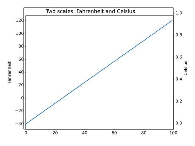
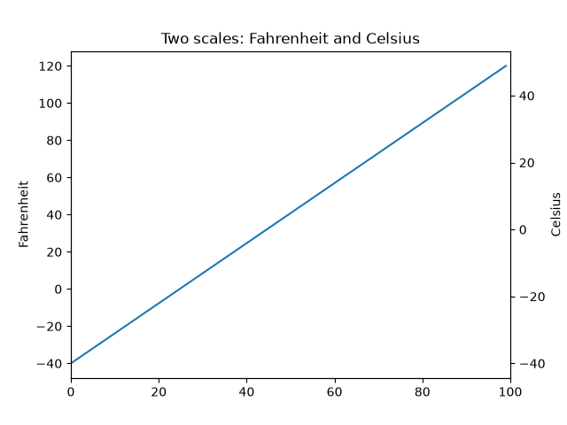
subplots_axes_and_figures/figure_size_units
==============================
Source
""" ============================== Figure size in different units ============================== The native figure size unit in Matplotlib is inches, deriving from print industry standards. However, users may need to specify their figures in other units like centimeters or pixels. This example illustrates how to do this efficiently. """ # sphinx_gallery_thumbnail_number = 2 import matplotlib.pyplot as plt text_kwargs = dict(ha='center', va='center', fontsize=28, color='C1') # %% # Figure size in inches (default) # ------------------------------- # plt.subplots(figsize=(6, 2)) plt.text(0.5, 0.5, '6 inches x 2 inches', **text_kwargs) plt.show() # %% # Figure size in centimeter # ------------------------- # Multiplying centimeter-based numbers with a conversion factor from cm to # inches, gives the right numbers. Naming the conversion factor ``cm`` makes # the conversion almost look like appending a unit to the number, which is # nicely readable. # cm = 1/2.54 # centimeters in inches plt.subplots(figsize=(15*cm, 5*cm)) plt.text(0.5, 0.5, '15cm x 5cm', **text_kwargs) plt.show() # %% # Figure size in pixel # -------------------- # Similarly, one can use a conversion from pixels. # # Note that you could break this if you use `~.pyplot.savefig` with a # different explicit dpi value. # px = 1/plt.rcParams['figure.dpi'] # pixel in inches plt.subplots(figsize=(600*px, 200*px)) plt.text(0.5, 0.5, '600px x 200px', **text_kwargs) plt.show() # %% # Quick interactive work is usually rendered to the screen, making pixels a # good size of unit. But defining the conversion factor may feel a little # tedious for quick iterations. # # Because of the default ``rcParams['figure.dpi'] = 100``, one can mentally # divide the needed pixel value by 100 [#]_: # plt.subplots(figsize=(6, 2)) plt.text(0.5, 0.5, '600px x 200px', **text_kwargs) plt.show() # %% # .. [#] Unfortunately, this does not work well for the ``matplotlib inline`` # backend in Jupyter because that backend saves the figure # with ``bbox_inches='tight'``, which crops the figure and makes the # actual size unpredictable. # %% # # .. admonition:: References # # The use of the following functions, methods, classes and modules is shown # in this example: # # - `matplotlib.pyplot.figure` # - `matplotlib.pyplot.subplots` # - `matplotlib.pyplot.subplot_mosaic` # # .. tags:: # # component: figure # styling: size # level: beginner
subplots_axes_and_figures/figure_title
=============================================
Source
"""
=============================================
Figure labels: suptitle, supxlabel, supylabel
=============================================
Each Axes can have a title (or actually three - one each with *loc* "left",
"center", and "right"), but is sometimes desirable to give a whole figure
(or `.SubFigure`) an overall title, using `.Figure.suptitle`.
We can also add figure-level x- and y-labels using `.Figure.supxlabel` and
`.Figure.supylabel`.
"""
import matplotlib.pyplot as plt
import numpy as np
from matplotlib.cbook import get_sample_data
x = np.linspace(0.0, 5.0, 501)
fig, (ax1, ax2) = plt.subplots(1, 2, layout='constrained', sharey=True)
ax1.plot(x, np.cos(6*x) * np.exp(-x))
ax1.set_title('damped')
ax1.set_xlabel('time (s)')
ax1.set_ylabel('amplitude')
ax2.plot(x, np.cos(6*x))
ax2.set_xlabel('time (s)')
ax2.set_title('undamped')
fig.suptitle('Different types of oscillations', fontsize=16)
# %%
# A global x- or y-label can be set using the `.Figure.supxlabel` and
# `.Figure.supylabel` methods.
with get_sample_data('Stocks.csv') as file:
stocks = np.genfromtxt(
file, delimiter=',', names=True, dtype=None,
converters={0: lambda x: np.datetime64(x, 'D')}, skip_header=1)
fig, axs = plt.subplots(4, 2, figsize=(9, 5), layout='constrained',
sharex=True, sharey=True)
for nn, ax in enumerate(axs.flat):
column_name = stocks.dtype.names[1+nn]
y = stocks[column_name]
line, = ax.plot(stocks['Date'], y / np.nanmax(y), lw=2.5)
ax.set_title(column_name, fontsize='small', loc='left')
fig.supxlabel('Year')
fig.supylabel('Stock price relative to max')
plt.show()
# %%
# .. tags::
#
# component: figure
# component: title
# plot-type: line
# level: beginner
subplots_axes_and_figures/ganged_plots
=================
Source
""" ================= Adjacent subplots ================= To create plots that share a common axis (visually) you can set the hspace between the subplots to zero. Passing sharex=True when creating the subplots will automatically turn off all x ticks and labels except those on the bottom axis. In this example the plots share a common x-axis, but you can follow the same logic to supply a common y-axis. """ import matplotlib.pyplot as plt import numpy as np t = np.arange(0.0, 2.0, 0.01) s1 = np.sin(2 * np.pi * t) s2 = np.exp(-t) s3 = s1 * s2 fig, axs = plt.subplots(3, 1, sharex=True) # Remove vertical space between Axes fig.subplots_adjust(hspace=0) # Plot each graph, and manually set the y tick values axs[0].plot(t, s1) axs[0].set_yticks(np.arange(-0.9, 1.0, 0.4)) axs[0].set_ylim(-1, 1) axs[1].plot(t, s2) axs[1].set_yticks(np.arange(0.1, 1.0, 0.2)) axs[1].set_ylim(0, 1) axs[2].plot(t, s3) axs[2].set_yticks(np.arange(-0.9, 1.0, 0.4)) axs[2].set_ylim(-1, 1) plt.show() # %% # .. tags:: # # component: subplot # plot-type: line # level: beginner
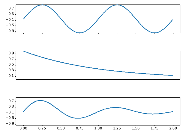
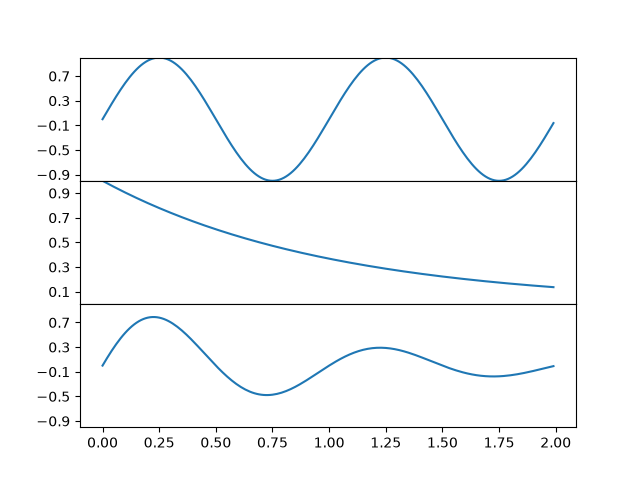
subplots_axes_and_figures/geo_demo
======================
Source
"""
======================
Geographic Projections
======================
This shows 4 possible geographic projections. Cartopy_ supports more
projections.
.. _Cartopy: https://cartopy.readthedocs.io
"""
import matplotlib.pyplot as plt
# %%
plt.figure()
plt.subplot(projection="aitoff")
plt.title("Aitoff")
plt.grid(True)
# %%
plt.figure()
plt.subplot(projection="hammer")
plt.title("Hammer")
plt.grid(True)
# %%
plt.figure()
plt.subplot(projection="lambert")
plt.title("Lambert")
plt.grid(True)
# %%
plt.figure()
plt.subplot(projection="mollweide")
plt.title("Mollweide")
plt.grid(True)
plt.show()
# %%
# .. tags::
#
# plot-type: specialty
# component: projection
# domain: cartography
subplots_axes_and_figures/gridspec_and_subplots
================================================
Source
"""
================================================
Combine two subplots using subplots and GridSpec
================================================
Sometimes we want to combine two subplots in an Axes layout created with
`~.Figure.subplots`. We can get the `~.gridspec.GridSpec` from the Axes
and then remove the covered Axes and fill the gap with a new bigger Axes.
Here we create a layout with the bottom two Axes in the last column combined.
To start with this layout (rather than removing the overlapping Axes) use
`~.pyplot.subplot_mosaic`.
See also :ref:`arranging_axes`.
"""
import matplotlib.pyplot as plt
fig, axs = plt.subplots(ncols=3, nrows=3)
gs = axs[1, 2].get_gridspec()
# remove the underlying Axes
for ax in axs[1:, -1]:
ax.remove()
axbig = fig.add_subplot(gs[1:, -1])
axbig.annotate('Big Axes \nGridSpec[1:, -1]', (0.1, 0.5),
xycoords='axes fraction', va='center')
fig.tight_layout()
plt.show()
# %%
# .. tags::
#
# component: subplot
# level: beginner
subplots_axes_and_figures/gridspec_customization
========================================
Source
"""
========================================
GridSpec with variable sizes and spacing
========================================
This example demonstrates the use of `.GridSpec` to generate subplots,
the control of the relative sizes of subplots with *width_ratios* and
*height_ratios*, and the control of the spacing around and between subplots
using subplot params (*left*, *right*, *bottom*, *top*, *wspace*, and
*hspace*).
.. redirect-from:: /gallery/userdemo/demo_gridspec03
"""
import matplotlib.pyplot as plt
from matplotlib.gridspec import GridSpec
def annotate_axes(fig):
for i, ax in enumerate(fig.axes):
ax.text(0.5, 0.5, "ax%d" % (i+1), va="center", ha="center")
ax.tick_params(labelbottom=False, labelleft=False)
fig = plt.figure()
fig.suptitle("Controlling subplot sizes with width_ratios and height_ratios")
gs = GridSpec(2, 2, width_ratios=[1, 2], height_ratios=[4, 1])
ax1 = fig.add_subplot(gs[0])
ax2 = fig.add_subplot(gs[1])
ax3 = fig.add_subplot(gs[2])
ax4 = fig.add_subplot(gs[3])
annotate_axes(fig)
# %%
fig = plt.figure()
fig.suptitle("Controlling spacing around and between subplots")
gs1 = GridSpec(3, 3, left=0.05, right=0.48, wspace=0.05)
ax1 = fig.add_subplot(gs1[:-1, :])
ax2 = fig.add_subplot(gs1[-1, :-1])
ax3 = fig.add_subplot(gs1[-1, -1])
gs2 = GridSpec(3, 3, left=0.55, right=0.98, hspace=0.05)
ax4 = fig.add_subplot(gs2[:, :-1])
ax5 = fig.add_subplot(gs2[:-1, -1])
ax6 = fig.add_subplot(gs2[-1, -1])
annotate_axes(fig)
plt.show()
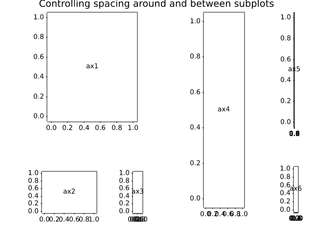
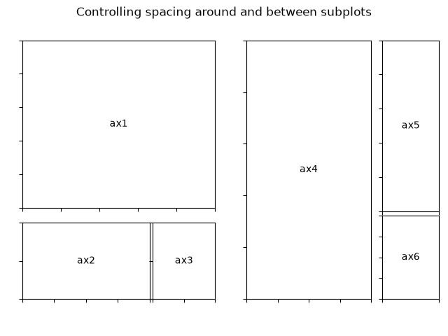
subplots_axes_and_figures/gridspec_multicolumn
=============================================
Source
"""
=============================================
Gridspec for multi-column/row subplot layouts
=============================================
`.GridSpec` is a flexible way to layout
subplot grids. Here is an example with a 3x3 grid, and
axes spanning all three columns, two columns, and two rows.
"""
import matplotlib.pyplot as plt
from matplotlib.gridspec import GridSpec
def format_axes(fig):
for i, ax in enumerate(fig.axes):
ax.text(0.5, 0.5, "ax%d" % (i+1), va="center", ha="center")
ax.tick_params(labelbottom=False, labelleft=False)
fig = plt.figure(layout="constrained")
gs = GridSpec(3, 3, figure=fig)
ax1 = fig.add_subplot(gs[0, :])
# identical to ax1 = plt.subplot(gs.new_subplotspec((0, 0), colspan=3))
ax2 = fig.add_subplot(gs[1, :-1])
ax3 = fig.add_subplot(gs[1:, -1])
ax4 = fig.add_subplot(gs[-1, 0])
ax5 = fig.add_subplot(gs[-1, -2])
fig.suptitle("GridSpec")
format_axes(fig)
plt.show()
# %%
# .. tags::
#
# component: subplot
# level: intermediate
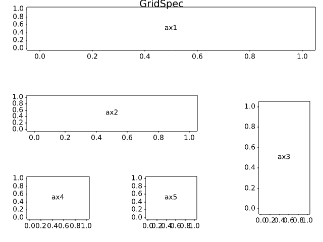
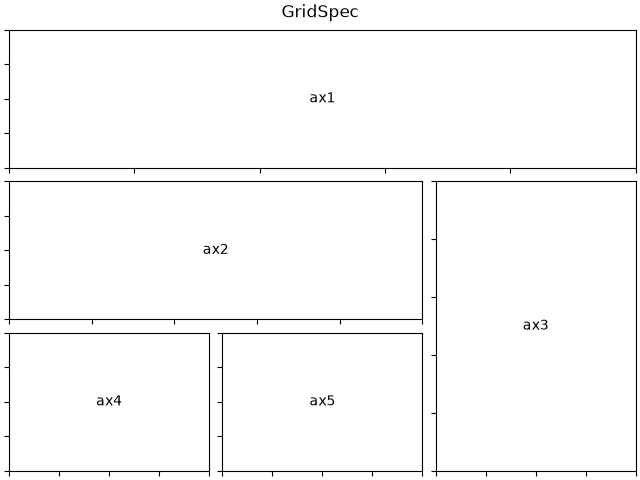
subplots_axes_and_figures/gridspec_nested
.. redirect-from:: /gallery/userdemo/demo_gridspec06
Source
"""
.. redirect-from:: /gallery/userdemo/demo_gridspec06
================
Nested Gridspecs
================
GridSpecs can be nested, so that a subplot from a parent GridSpec can
set the position for a nested grid of subplots.
Note that the same functionality can be achieved more directly with
`~.Figure.subfigures`; see
:doc:`/gallery/subplots_axes_and_figures/subfigures`.
"""
import matplotlib.pyplot as plt
import matplotlib.gridspec as gridspec
def format_axes(fig):
for i, ax in enumerate(fig.axes):
ax.text(0.5, 0.5, "ax%d" % (i+1), va="center", ha="center")
ax.tick_params(labelbottom=False, labelleft=False)
# gridspec inside gridspec
fig = plt.figure()
gs0 = gridspec.GridSpec(1, 2, figure=fig)
gs00 = gridspec.GridSpecFromSubplotSpec(3, 3, subplot_spec=gs0[0])
ax1 = fig.add_subplot(gs00[:-1, :])
ax2 = fig.add_subplot(gs00[-1, :-1])
ax3 = fig.add_subplot(gs00[-1, -1])
# the following syntax does the same as the GridSpecFromSubplotSpec call above:
gs01 = gs0[1].subgridspec(3, 3)
ax4 = fig.add_subplot(gs01[:, :-1])
ax5 = fig.add_subplot(gs01[:-1, -1])
ax6 = fig.add_subplot(gs01[-1, -1])
plt.suptitle("GridSpec Inside GridSpec")
format_axes(fig)
plt.show()
# %%
# .. tags::
#
# component: subplot
# level: intermediate
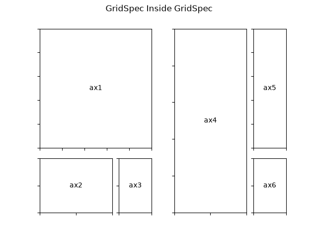
subplots_axes_and_figures/invert_axes
=============
Source
"""
=============
Inverted axis
=============
This example demonstrates two ways to invert the direction of an axis:
- If you want to set *explicit axis limits* anyway, e.g. via `~.Axes.set_xlim`, you
can swap the limit values: ``set_xlim(4, 0)`` instead of ``set_xlim(0, 4)``.
- Use `.Axis.set_inverted` if you only want to invert the axis *without modifying
the limits*, i.e. keep existing limits or existing autoscaling behavior.
"""
import matplotlib.pyplot as plt
import numpy as np
x = np.arange(0.01, 4.0, 0.01)
y = np.exp(-x)
fig, (ax1, ax2) = plt.subplots(1, 2, figsize=(6.4, 4), layout="constrained")
fig.suptitle('Inverted axis with ...')
ax1.plot(x, y)
ax1.set_xlim(4, 0) # inverted fixed limits
ax1.set_title('fixed limits: set_xlim(4, 0)')
ax1.set_xlabel('decreasing x ⟶')
ax1.grid(True)
ax2.plot(x, y)
ax2.xaxis.set_inverted(True) # inverted axis with autoscaling
ax2.set_title('autoscaling: set_inverted(True)')
ax2.set_xlabel('decreasing x ⟶')
ax2.grid(True)
plt.show()
# %%
# .. tags::
#
# component: axis
# plot-type: line
# level: beginner
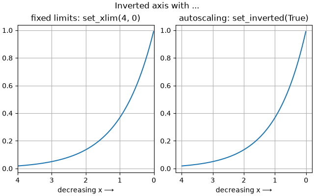
subplots_axes_and_figures/multiple_figs_demo
=================================
Source
"""
=================================
Manage multiple figures in pyplot
=================================
`matplotlib.pyplot` uses the concept of a *current figure* and *current Axes*.
Figures are identified via a figure number that is passed to `~.pyplot.figure`.
The figure with the given number is set as *current figure*. Additionally, if
no figure with the number exists, a new one is created.
.. note::
We discourage working with multiple figures through the implicit pyplot
interface because managing the *current figure* is cumbersome and
error-prone. Instead, we recommend using the explicit approach and call
methods on Figure and Axes instances. See :ref:`api_interfaces` for an
explanation of the trade-offs between the implicit and explicit interfaces.
"""
import matplotlib.pyplot as plt
import numpy as np
t = np.arange(0.0, 2.0, 0.01)
s1 = np.sin(2*np.pi*t)
s2 = np.sin(4*np.pi*t)
# %%
# Create figure 1
plt.figure(1)
plt.subplot(211)
plt.plot(t, s1)
plt.subplot(212)
plt.plot(t, 2*s1)
# %%
# Create figure 2
plt.figure(2)
plt.plot(t, s2)
# %%
# Now switch back to figure 1 and make some changes
plt.figure(1)
plt.subplot(211)
plt.plot(t, s2, 's')
ax = plt.gca()
ax.set_xticklabels([])
plt.show()
# %%
# .. tags:: component: figure, plot-type: line
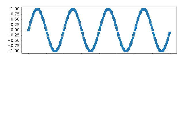
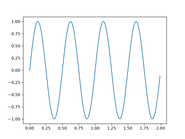
subplots_axes_and_figures/multiple_yaxis_with_spines
===========================
Source
r"""
===========================
Multiple y-axis with Spines
===========================
Create multiple y axes with a shared x-axis. This is done by creating
a `~.axes.Axes.twinx` Axes, turning all spines but the right one invisible
and offset its position using `~.spines.Spine.set_position`.
Note that this approach uses `matplotlib.axes.Axes` and their
`~matplotlib.spines.Spine`\s. Alternative approaches using non-standard Axes
are shown in the :doc:`/gallery/axisartist/demo_parasite_axes` and
:doc:`/gallery/axisartist/demo_parasite_axes2` examples.
.. redirect-from:: /gallery/spines/multiple_yaxis_with_spines
"""
import matplotlib.pyplot as plt
fig, ax = plt.subplots()
fig.subplots_adjust(right=0.75)
twin1 = ax.twinx()
twin2 = ax.twinx()
# Offset the right spine of twin2. The ticks and label have already been
# placed on the right by twinx above.
twin2.spines.right.set_position(("axes", 1.2))
p1, = ax.plot([0, 1, 2], [0, 1, 2], "C0", label="Density")
p2, = twin1.plot([0, 1, 2], [0, 3, 2], "C1", label="Temperature")
p3, = twin2.plot([0, 1, 2], [50, 30, 15], "C2", label="Velocity")
ax.set(xlim=(0, 2), ylim=(0, 2), xlabel="Distance", ylabel="Density")
twin1.set(ylim=(0, 4), ylabel="Temperature")
twin2.set(ylim=(1, 65), ylabel="Velocity")
ax.yaxis.label.set_color(p1.get_color())
twin1.yaxis.label.set_color(p2.get_color())
twin2.yaxis.label.set_color(p3.get_color())
ax.tick_params(axis='y', colors=p1.get_color())
twin1.tick_params(axis='y', colors=p2.get_color())
twin2.tick_params(axis='y', colors=p3.get_color())
ax.legend(handles=[p1, p2, p3])
plt.show()
# %%
# .. tags:: component: spines
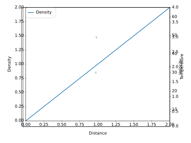
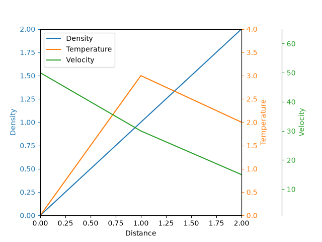
subplots_axes_and_figures/secondary_axis
==============
Source
"""
==============
Secondary Axis
==============
Sometimes we want a secondary axis on a plot, for instance to convert
radians to degrees on the same plot. We can do this by making a child
axes with only one axis visible via `.axes.Axes.secondary_xaxis` and
`.axes.Axes.secondary_yaxis`. This secondary axis can have a different scale
than the main axis by providing both a forward and an inverse conversion
function in a tuple to the *functions* keyword argument:
See also :doc:`/gallery/subplots_axes_and_figures/two_scales` for the case
where two scales are not related to one another, but independent.
"""
import datetime
import matplotlib.pyplot as plt
import numpy as np
import matplotlib.dates as mdates
fig, ax = plt.subplots(layout='constrained')
x = np.arange(0, 360, 1)
y = np.sin(2 * x * np.pi / 180)
ax.plot(x, y)
ax.set_xlabel('angle [degrees]')
ax.set_ylabel('signal')
ax.set_title('Sine wave')
def deg2rad(x):
return x * np.pi / 180
def rad2deg(x):
return x * 180 / np.pi
secax = ax.secondary_xaxis('top', functions=(deg2rad, rad2deg))
secax.set_xlabel('angle [rad]')
plt.show()
# %%
# By default, the secondary axis is drawn in the Axes coordinate space.
# We can also provide a custom transform to place it in a different
# coordinate space. Here we put the axis at Y = 0 in data coordinates.
fig, ax = plt.subplots(layout='constrained')
x = np.arange(0, 10)
np.random.seed(19680801)
y = np.random.randn(len(x))
ax.plot(x, y)
ax.set_xlabel('X')
ax.set_ylabel('Y')
ax.set_title('Random data')
# Pass ax.transData as a transform to place the axis relative to our data
secax = ax.secondary_xaxis(0, transform=ax.transData)
secax.set_xlabel('Axis at Y = 0')
plt.show()
# %%
# Here is the case of converting from wavenumber to wavelength in a
# log-log scale.
#
# .. note::
#
# In this case, the xscale of the parent is logarithmic, so the child is
# made logarithmic as well.
fig, ax = plt.subplots(layout='constrained')
x = np.arange(0.02, 1, 0.02)
np.random.seed(19680801)
y = np.random.randn(len(x)) ** 2
ax.loglog(x, y)
ax.set_xlabel('f [Hz]')
ax.set_ylabel('PSD')
ax.set_title('Random spectrum')
def one_over(x):
"""Vectorized 1/x, treating x==0 manually"""
x = np.array(x, float)
near_zero = np.isclose(x, 0)
x[near_zero] = np.inf
x[~near_zero] = 1 / x[~near_zero]
return x
# the function "1/x" is its own inverse
inverse = one_over
secax = ax.secondary_xaxis('top', functions=(one_over, inverse))
secax.set_xlabel('period [s]')
plt.show()
# %%
# Sometime we want to relate the axes in a transform that is ad-hoc from the data, and
# is derived empirically. Or, one axis could be a complicated nonlinear function of the
# other. In these cases we can set the forward and inverse transform functions to be
# linear interpolations from the one set of independent variables to the other.
#
# .. note::
#
# In order to properly handle the data margins, the mapping functions
# (``forward`` and ``inverse`` in this example) need to be defined beyond the
# nominal plot limits. This condition can be enforced by extending the
# interpolation beyond the plotted values, both to the left and the right,
# see ``x1n`` and ``x2n`` below.
fig, ax = plt.subplots(layout='constrained')
x1_vals = np.arange(2, 11, 0.4)
# second independent variable is a nonlinear function of the other.
x2_vals = x1_vals ** 2
ydata = 50.0 + 20 * np.random.randn(len(x1_vals))
ax.plot(x1_vals, ydata, label='Plotted data')
ax.plot(x1_vals, x2_vals, label=r'$x_2 = x_1^2$')
ax.set_xlabel(r'$x_1$')
ax.legend()
# the forward and inverse functions must be defined on the complete visible axis range
x1n = np.linspace(0, 20, 201)
x2n = x1n**2
def forward(x):
return np.interp(x, x1n, x2n)
def inverse(x):
return np.interp(x, x2n, x1n)
# use axvline to prove that the derived secondary axis is correctly plotted
ax.axvline(np.sqrt(40), color="grey", ls="--")
ax.axvline(10, color="grey", ls="--")
secax = ax.secondary_xaxis('top', functions=(forward, inverse))
secax.set_xticks([10, 20, 40, 60, 80, 100])
secax.set_xlabel(r'$x_2$')
plt.show()
# %%
# A final example translates np.datetime64 to yearday on the x axis and
# from Celsius to Fahrenheit on the y axis. Note the addition of a
# third y axis, and that it can be placed using a float for the
# location argument
dates = [datetime.datetime(2018, 1, 1) + datetime.timedelta(hours=k * 6)
for k in range(240)]
temperature = np.random.randn(len(dates)) * 4 + 6.7
fig, ax = plt.subplots(layout='constrained')
ax.plot(dates, temperature)
ax.set_ylabel(r'$T\ [^oC]$')
ax.xaxis.set_tick_params(rotation=70)
def date2yday(x):
"""Convert matplotlib datenum to days since 2018-01-01."""
y = x - mdates.date2num(datetime.datetime(2018, 1, 1))
return y
def yday2date(x):
"""Return a matplotlib datenum for *x* days after 2018-01-01."""
y = x + mdates.date2num(datetime.datetime(2018, 1, 1))
return y
secax_x = ax.secondary_xaxis('top', functions=(date2yday, yday2date))
secax_x.set_xlabel('yday [2018]')
def celsius_to_fahrenheit(x):
return x * 1.8 + 32
def fahrenheit_to_celsius(x):
return (x - 32) / 1.8
secax_y = ax.secondary_yaxis(
'right', functions=(celsius_to_fahrenheit, fahrenheit_to_celsius))
secax_y.set_ylabel(r'$T\ [^oF]$')
def celsius_to_anomaly(x):
return (x - np.mean(temperature))
def anomaly_to_celsius(x):
return (x + np.mean(temperature))
# use of a float for the position:
secax_y2 = ax.secondary_yaxis(
1.2, functions=(celsius_to_anomaly, anomaly_to_celsius))
secax_y2.set_ylabel(r'$T - \overline{T}\ [^oC]$')
plt.show()
# %%
#
# .. admonition:: References
#
# The use of the following functions, methods, classes and modules is shown
# in this example:
#
# - `matplotlib.axes.Axes.secondary_xaxis`
# - `matplotlib.axes.Axes.secondary_yaxis`
#
# .. tags::
#
# component: axis
# plot-type: line
# level: beginner
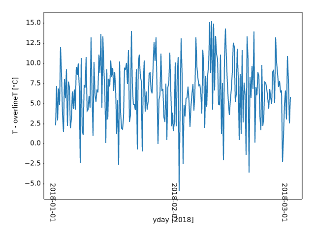
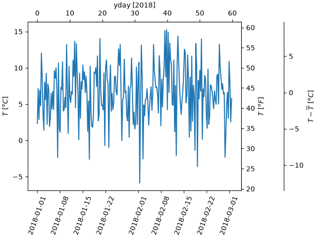
subplots_axes_and_figures/shared_axis_demo
===========
Source
"""
===========
Shared axis
===========
Use axis sharing when you want to compare data across multiple subplots, and want to
ensure they are on the same scale. To do so, pass ``sharex=True`` and/or ``sharey=True``
to `~.pyplot.subplots`.
This ensures the x- or y-axis limits are synchronized across the subplots. Autoscaling
considers the data on all Axes; therefore, any limit changes, including interactive zoom
and pan, will affect all shared axes.
The plot below illustrates this by showing two different time-series and using *sharex*
to ensure the times are aligned.
For more info see :ref:`sharing-axes`.
.. redirect-from:: /gallery/subplots_axes_and_figures/share_axis_lims_views
"""
import matplotlib.pyplot as plt
import numpy as np
t1 = np.linspace(0, 8, 201)
y1 = np.sin(2 * np.pi * t1)
t2 = np.linspace(2, 10, 201)
y2 = 20 * np.cos(2 * np.pi * t2)**2 * np.exp(-0.3*t2)
fig, (ax1, ax2) = plt.subplots(2, sharex=True)
ax1.plot(t1, y1)
ax1.set_ylabel("Signal 1")
ax2.plot(t2, y2)
ax2.set_ylabel("Signal 2")
ax2.set_xlabel("Time (s)")
plt.show()
# %%
# .. tags::
#
# component: axis
# plot-type: line
# level: beginner
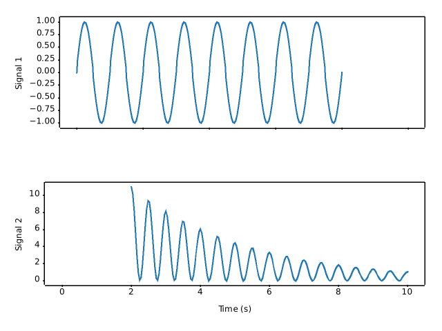
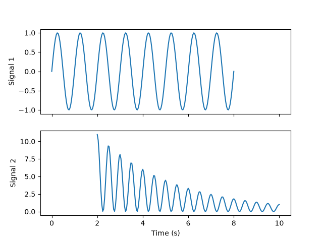
subplots_axes_and_figures/subfigures
=================
Source
"""
=================
Figure subfigures
=================
Sometimes it is desirable to have a figure with two different layouts in it.
This can be achieved with
:doc:`nested gridspecs</gallery/subplots_axes_and_figures/gridspec_nested>`,
but having a virtual figure with its own artists is helpful, so
Matplotlib also has "subfigures", accessed by calling
`matplotlib.figure.Figure.add_subfigure` in a way that is analogous to
`matplotlib.figure.Figure.add_subplot`, or
`matplotlib.figure.Figure.subfigures` to make an array of subfigures. Note
that subfigures can also have their own child subfigures.
"""
import matplotlib.pyplot as plt
import numpy as np
def example_plot(ax, fontsize=12, hide_labels=False):
pc = ax.pcolormesh(np.random.randn(30, 30), vmin=-2.5, vmax=2.5)
if not hide_labels:
ax.set_xlabel('x-label', fontsize=fontsize)
ax.set_ylabel('y-label', fontsize=fontsize)
ax.set_title('Title', fontsize=fontsize)
return pc
np.random.seed(19680808)
# gridspec inside gridspec
fig = plt.figure(layout='constrained', figsize=(10, 4))
subfigs = fig.subfigures(1, 2, wspace=0.07)
axsLeft = subfigs[0].subplots(1, 2, sharey=True)
subfigs[0].set_facecolor('0.75')
for ax in axsLeft:
pc = example_plot(ax)
subfigs[0].suptitle('Left plots', fontsize='x-large')
subfigs[0].colorbar(pc, shrink=0.6, ax=axsLeft, location='bottom')
axsRight = subfigs[1].subplots(3, 1, sharex=True)
for nn, ax in enumerate(axsRight):
pc = example_plot(ax, hide_labels=True)
if nn == 2:
ax.set_xlabel('xlabel')
if nn == 1:
ax.set_ylabel('ylabel')
subfigs[1].set_facecolor('0.85')
subfigs[1].colorbar(pc, shrink=0.6, ax=axsRight)
subfigs[1].suptitle('Right plots', fontsize='x-large')
fig.suptitle('Figure suptitle', fontsize='xx-large')
plt.show()
# %%
# It is possible to mix subplots and subfigures using
# `matplotlib.figure.Figure.add_subfigure`. This requires getting
# the gridspec that the subplots are laid out on.
fig, axs = plt.subplots(2, 3, layout='constrained', figsize=(10, 4))
gridspec = axs[0, 0].get_subplotspec().get_gridspec()
# clear the left column for the subfigure:
for a in axs[:, 0]:
a.remove()
# plot data in remaining Axes:
for a in axs[:, 1:].flat:
a.plot(np.arange(10))
# make the subfigure in the empty gridspec slots:
subfig = fig.add_subfigure(gridspec[:, 0])
axsLeft = subfig.subplots(1, 2, sharey=True)
subfig.set_facecolor('0.75')
for ax in axsLeft:
pc = example_plot(ax)
subfig.suptitle('Left plots', fontsize='x-large')
subfig.colorbar(pc, shrink=0.6, ax=axsLeft, location='bottom')
fig.suptitle('Figure suptitle', fontsize='xx-large')
plt.show()
# %%
# Subfigures can have different widths and heights. This is exactly the
# same example as the first example, but *width_ratios* has been changed:
fig = plt.figure(layout='constrained', figsize=(10, 4))
subfigs = fig.subfigures(1, 2, wspace=0.07, width_ratios=[2, 1])
axsLeft = subfigs[0].subplots(1, 2, sharey=True)
subfigs[0].set_facecolor('0.75')
for ax in axsLeft:
pc = example_plot(ax)
subfigs[0].suptitle('Left plots', fontsize='x-large')
subfigs[0].colorbar(pc, shrink=0.6, ax=axsLeft, location='bottom')
axsRight = subfigs[1].subplots(3, 1, sharex=True)
for nn, ax in enumerate(axsRight):
pc = example_plot(ax, hide_labels=True)
if nn == 2:
ax.set_xlabel('xlabel')
if nn == 1:
ax.set_ylabel('ylabel')
subfigs[1].set_facecolor('0.85')
subfigs[1].colorbar(pc, shrink=0.6, ax=axsRight)
subfigs[1].suptitle('Right plots', fontsize='x-large')
fig.suptitle('Figure suptitle', fontsize='xx-large')
plt.show()
# %%
# Subfigures can be also be nested:
fig = plt.figure(layout='constrained', figsize=(10, 8))
fig.suptitle('fig')
subfigs = fig.subfigures(1, 2, wspace=0.07)
subfigs[0].set_facecolor('coral')
subfigs[0].suptitle('subfigs[0]')
subfigs[1].set_facecolor('coral')
subfigs[1].suptitle('subfigs[1]')
subfigsnest = subfigs[0].subfigures(2, 1, height_ratios=[1, 1.4])
subfigsnest[0].suptitle('subfigsnest[0]')
subfigsnest[0].set_facecolor('r')
axsnest0 = subfigsnest[0].subplots(1, 2, sharey=True)
for nn, ax in enumerate(axsnest0):
pc = example_plot(ax, hide_labels=True)
subfigsnest[0].colorbar(pc, ax=axsnest0)
subfigsnest[1].suptitle('subfigsnest[1]')
subfigsnest[1].set_facecolor('g')
axsnest1 = subfigsnest[1].subplots(3, 1, sharex=True)
axsRight = subfigs[1].subplots(2, 2)
plt.show()
# %%
# .. tags::
#
# component: figure
# plot-type: pcolormesh
# level: intermediate
subplots_axes_and_figures/subplot
=================
Source
"""
=================
Multiple subplots
=================
Simple demo with multiple subplots.
For more options, see :doc:`/gallery/subplots_axes_and_figures/subplots_demo`.
.. redirect-from:: /gallery/subplots_axes_and_figures/subplot_demo
"""
import matplotlib.pyplot as plt
import numpy as np
# Create some fake data.
x1 = np.linspace(0.0, 5.0)
y1 = np.cos(2 * np.pi * x1) * np.exp(-x1)
x2 = np.linspace(0.0, 2.0)
y2 = np.cos(2 * np.pi * x2)
# %%
# `~.pyplot.subplots()` is the recommended method to generate simple subplot
# arrangements:
fig, (ax1, ax2) = plt.subplots(2, 1)
fig.suptitle('A tale of 2 subplots')
ax1.plot(x1, y1, 'o-')
ax1.set_ylabel('Damped oscillation')
ax2.plot(x2, y2, '.-')
ax2.set_xlabel('time (s)')
ax2.set_ylabel('Undamped')
plt.show()
# %%
# Subplots can also be generated one at a time using `~.pyplot.subplot()`:
plt.subplot(2, 1, 1)
plt.plot(x1, y1, 'o-')
plt.title('A tale of 2 subplots')
plt.ylabel('Damped oscillation')
plt.subplot(2, 1, 2)
plt.plot(x2, y2, '.-')
plt.xlabel('time (s)')
plt.ylabel('Undamped')
plt.show()
# %%
# .. tags::
#
# component: subplot
# plot-type: line
# level: beginner
subplots_axes_and_figures/subplot2grid
============
Source
"""
============
subplot2grid
============
This example demonstrates the use of `.pyplot.subplot2grid` to generate
subplots. Using `.GridSpec`, as demonstrated in
:doc:`/gallery/subplots_axes_and_figures/gridspec_customization` is
generally preferred.
.. redirect-from:: /gallery/userdemo/demo_gridspec01
"""
import matplotlib.pyplot as plt
def annotate_axes(fig):
for i, ax in enumerate(fig.axes):
ax.text(0.5, 0.5, "ax%d" % (i+1), va="center", ha="center")
ax.tick_params(labelbottom=False, labelleft=False)
fig = plt.figure()
ax1 = plt.subplot2grid((3, 3), (0, 0), colspan=3)
ax2 = plt.subplot2grid((3, 3), (1, 0), colspan=2)
ax3 = plt.subplot2grid((3, 3), (1, 2), rowspan=2)
ax4 = plt.subplot2grid((3, 3), (2, 0))
ax5 = plt.subplot2grid((3, 3), (2, 1))
annotate_axes(fig)
plt.show()
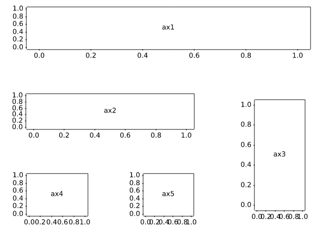
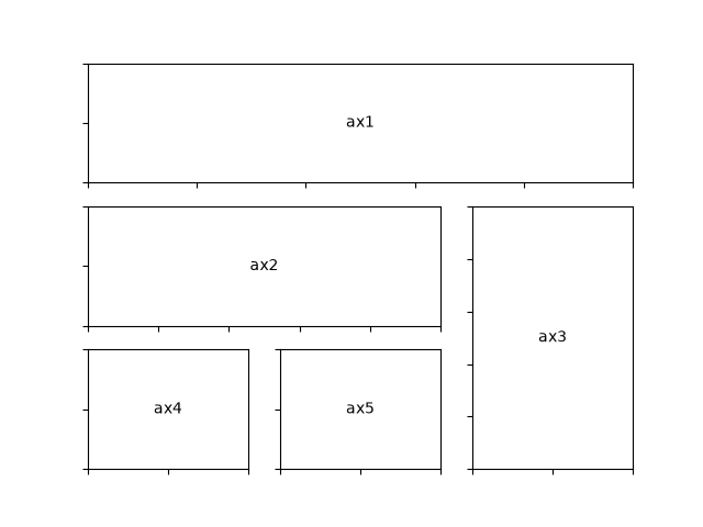
subplots_axes_and_figures/subplots_adjust
=============================
Source
""" ============================= Subplots spacings and margins ============================= Adjusting the spacing of margins and subplots using `.pyplot.subplots_adjust`. .. note:: There is also a tool window to adjust the margins and spacings of displayed figures interactively. It can be opened via the toolbar or by calling `.pyplot.subplot_tool`. .. redirect-from:: /gallery/subplots_axes_and_figures/subplot_toolbar """ import matplotlib.pyplot as plt import numpy as np # Fixing random state for reproducibility np.random.seed(19680801) plt.subplot(211) plt.imshow(np.random.random((100, 100))) plt.subplot(212) plt.imshow(np.random.random((100, 100))) plt.subplots_adjust(bottom=0.1, right=0.8, top=0.9) cax = plt.axes((0.85, 0.1, 0.075, 0.8)) plt.colorbar(cax=cax) plt.show() # %% # .. tags:: # # component: subplot # plot-type: imshow # level: beginner
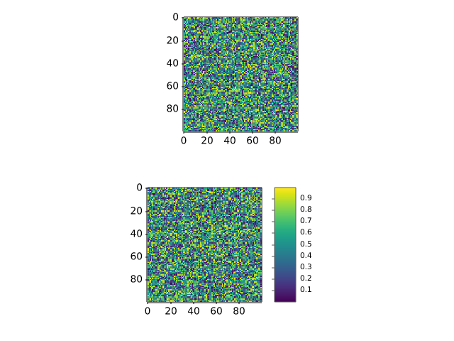
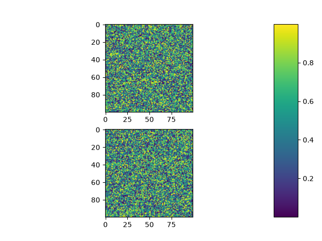
subplots_axes_and_figures/subplots_demo
===============================================
Source
"""
===============================================
Create multiple subplots using ``plt.subplots``
===============================================
`.pyplot.subplots` creates a figure and a grid of subplots with a single call,
while providing reasonable control over how the individual plots are created.
For more advanced use cases you can use `.GridSpec` for a more general subplot
layout or `.Figure.add_subplot` for adding subplots at arbitrary locations
within the figure.
"""
# sphinx_gallery_thumbnail_number = 11
import matplotlib.pyplot as plt
import numpy as np
# Some example data to display
x = np.linspace(0, 2 * np.pi, 400)
y = np.sin(x ** 2)
# %%
# A figure with just one subplot
# """"""""""""""""""""""""""""""
#
# ``subplots()`` without arguments returns a `.Figure` and a single
# `~.axes.Axes`.
#
# This is actually the simplest and recommended way of creating a single
# Figure and Axes.
fig, ax = plt.subplots()
ax.plot(x, y)
ax.set_title('A single plot')
# %%
# Stacking subplots in one direction
# """"""""""""""""""""""""""""""""""
#
# The first two optional arguments of `.pyplot.subplots` define the number of
# rows and columns of the subplot grid.
#
# When stacking in one direction only, the returned ``axs`` is a 1D numpy array
# containing the list of created Axes.
fig, axs = plt.subplots(2)
fig.suptitle('Vertically stacked subplots')
axs[0].plot(x, y)
axs[1].plot(x, -y)
# %%
# If you are creating just a few Axes, it's handy to unpack them immediately to
# dedicated variables for each Axes. That way, we can use ``ax1`` instead of
# the more verbose ``axs[0]``.
fig, (ax1, ax2) = plt.subplots(2)
fig.suptitle('Vertically stacked subplots')
ax1.plot(x, y)
ax2.plot(x, -y)
# %%
# To obtain side-by-side subplots, pass parameters ``1, 2`` for one row and two
# columns.
fig, (ax1, ax2) = plt.subplots(1, 2)
fig.suptitle('Horizontally stacked subplots')
ax1.plot(x, y)
ax2.plot(x, -y)
# %%
# Stacking subplots in two directions
# """""""""""""""""""""""""""""""""""
#
# When stacking in two directions, the returned ``axs`` is a 2D NumPy array.
#
# If you have to set parameters for each subplot it's handy to iterate over
# all subplots in a 2D grid using ``for ax in axs.flat:``.
fig, axs = plt.subplots(2, 2)
axs[0, 0].plot(x, y)
axs[0, 0].set_title('Axis [0, 0]')
axs[0, 1].plot(x, y, 'tab:orange')
axs[0, 1].set_title('Axis [0, 1]')
axs[1, 0].plot(x, -y, 'tab:green')
axs[1, 0].set_title('Axis [1, 0]')
axs[1, 1].plot(x, -y, 'tab:red')
axs[1, 1].set_title('Axis [1, 1]')
for ax in axs.flat:
ax.set(xlabel='x-label', ylabel='y-label')
# Hide x labels and tick labels for top plots and y ticks for right plots.
for ax in axs.flat:
ax.label_outer()
# %%
# You can use tuple-unpacking also in 2D to assign all subplots to dedicated
# variables:
fig, ((ax1, ax2), (ax3, ax4)) = plt.subplots(2, 2)
fig.suptitle('Sharing x per column, y per row')
ax1.plot(x, y)
ax2.plot(x, y**2, 'tab:orange')
ax3.plot(x, -y, 'tab:green')
ax4.plot(x, -y**2, 'tab:red')
for ax in fig.get_axes():
ax.label_outer()
# %%
# .. _sharing-axes:
#
# Sharing axes
# """"""""""""
#
# By default, each Axes is scaled individually. Thus, if the ranges are
# different the tick values of the subplots do not align.
fig, (ax1, ax2) = plt.subplots(2)
fig.suptitle('Axes values are scaled individually by default')
ax1.plot(x, y)
ax2.plot(x + 1, -y)
# %%
# You can use *sharex* or *sharey* to align the horizontal or vertical axis.
fig, (ax1, ax2) = plt.subplots(2, sharex=True)
fig.suptitle('Aligning x-axis using sharex')
ax1.plot(x, y)
ax2.plot(x + 1, -y)
# %%
# Setting *sharex* or *sharey* to ``True`` enables global sharing across the
# whole grid, i.e. also the y-axes of vertically stacked subplots have the
# same scale when using ``sharey=True``.
fig, axs = plt.subplots(3, sharex=True, sharey=True)
fig.suptitle('Sharing both axes')
axs[0].plot(x, y ** 2)
axs[1].plot(x, 0.3 * y, 'o')
axs[2].plot(x, y, '+')
# %%
# For subplots that are sharing axes one set of tick labels is enough. Tick
# labels of inner Axes are automatically removed by *sharex* and *sharey*.
# You can selectively restore them using `~.axes.Axes.tick_params`.
fig, axs = plt.subplots(3, sharex=True, sharey=True)
fig.suptitle('Restored xtick labels on to Axes')
axs[0].plot(x, y ** 2)
axs[1].plot(x, 0.3 * y, 'o')
axs[2].plot(x, y, '+')
axs[0].tick_params(labelbottom=True)
# %%
# It is also possible to remove the empty space between the subplots.
# To precisely control the positioning of the subplots, one can explicitly
# create a `.GridSpec` with `.Figure.add_gridspec`, and then call its
# `~.GridSpecBase.subplots` method. For example, we can reduce the height
# between vertical subplots using ``add_gridspec(hspace=0)``.
#
# `.label_outer` is a handy method to remove labels and ticks from subplots
# that are not at the edge of the grid.
fig = plt.figure()
gs = fig.add_gridspec(3, hspace=0)
axs = gs.subplots(sharex=True, sharey=True)
fig.suptitle('Sharing both axes')
axs[0].plot(x, y ** 2)
axs[1].plot(x, 0.3 * y, 'o')
axs[2].plot(x, y, '+')
# Hide x labels and tick labels for all but bottom plot.
for ax in axs:
ax.label_outer()
# %%
# Apart from ``True`` and ``False``, both *sharex* and *sharey* accept the
# values 'row' and 'col' to share the values only per row or column.
fig = plt.figure()
gs = fig.add_gridspec(2, 2, hspace=0, wspace=0)
(ax1, ax2), (ax3, ax4) = gs.subplots(sharex='col', sharey='row')
fig.suptitle('Sharing x per column, y per row')
ax1.plot(x, y)
ax2.plot(x, y**2, 'tab:orange')
ax3.plot(x + 1, -y, 'tab:green')
ax4.plot(x + 2, -y**2, 'tab:red')
for ax in fig.get_axes():
ax.label_outer()
# %%
# If you want a more complex sharing structure, you can first create the
# grid of Axes with no sharing, and then call `.axes.Axes.sharex` or
# `.axes.Axes.sharey` to add sharing info a posteriori.
fig, axs = plt.subplots(2, 2)
axs[0, 0].plot(x, y)
axs[0, 0].set_title("main")
axs[1, 0].plot(x, y**2)
axs[1, 0].set_title("shares x with main")
axs[1, 0].sharex(axs[0, 0])
axs[0, 1].plot(x + 1, y + 1)
axs[0, 1].set_title("unrelated")
axs[1, 1].plot(x + 2, y + 2)
axs[1, 1].set_title("also unrelated")
fig.tight_layout()
# %%
# Polar Axes
# """"""""""
#
# The parameter *subplot_kw* of `.pyplot.subplots` controls the subplot
# properties (see also `.Figure.add_subplot`). In particular, this can be used
# to create a grid of polar Axes.
fig, (ax1, ax2) = plt.subplots(1, 2, subplot_kw=dict(projection='polar'))
ax1.plot(x, y)
ax2.plot(x, y ** 2)
plt.show()
# %%
# .. tags::
#
# component: subplot,
# component: axes,
# component: axis
# plot-type: line,
# plot-type: polar
# level: beginner
# purpose: showcase
subplots_axes_and_figures/twin_axes_zorder
===========================
Source
"""
===========================
Twin Axes with delta_zorder
===========================
`~matplotlib.axes.Axes.twinx` and `~matplotlib.axes.Axes.twiny` accept a
*delta_zorder* keyword argument (a relative offset added to the original Axes'
zorder) that controls whether the twin Axes is drawn in front of or behind the
original Axes.
Matplotlib also automatically manages background patch visibility for twinned
Axes groups so that only the bottom-most Axes has a visible background patch
(respecting ``frameon``). This avoids the background of a higher-zorder twin
Axes covering artists drawn on the underlying Axes.
"""
import matplotlib.pyplot as plt
import numpy as np
x = np.linspace(0, 10, 400)
y_main = np.sin(x)
y_twin = 0.4 * np.cos(x) + 0.6
fig, ax = plt.subplots()
# Put the twin Axes behind the original Axes (relative to the original zorder).
ax2 = ax.twinx(delta_zorder=-1)
# Draw something broad on the twin Axes so that the stacking is obvious.
ax2.fill_between(x, 0, y_twin, color="C1", alpha=0.35, label="twin fill")
ax2.plot(x, y_twin, color="C1", lw=6, alpha=0.8)
# Draw overlapping artists on the main Axes; they appear on top.
ax.scatter(x[::8], y_main[::8], s=35, color="C0", edgecolor="k", linewidth=0.5,
zorder=3, label="main scatter")
ax.plot(x, y_main, color="C0", lw=4)
ax.set_xlabel("x")
ax.set_ylabel("main y")
ax2.set_ylabel("twin y")
ax.set_title("Twin Axes drawn behind the main Axes using delta_zorder")
fig.tight_layout()
plt.show()
subplots_axes_and_figures/two_scales
===========================
Source
"""
===========================
Plots with different scales
===========================
Two plots on the same Axes with different left and right scales.
The trick is to use *two different Axes* that share the same *x* axis.
You can use separate `matplotlib.ticker` formatters and locators as
desired since the two Axes are independent.
Such Axes are generated by calling the `.Axes.twinx` method. Likewise,
`.Axes.twiny` is available to generate Axes that share a *y* axis but
have different top and bottom scales.
See also :doc:`/gallery/subplots_axes_and_figures/secondary_axis` for the case
where the two scales are not independent, but related (e.g., the same quantity
in two different units).
"""
import matplotlib.pyplot as plt
import numpy as np
# Create some mock data
t = np.arange(0.01, 10.0, 0.01)
data1 = np.exp(t)
data2 = np.sin(2 * np.pi * t)
fig, ax1 = plt.subplots()
color = 'tab:red'
ax1.set_xlabel('time (s)')
ax1.set_ylabel('exp', color=color)
ax1.plot(t, data1, color=color)
ax1.tick_params(axis='y', labelcolor=color)
ax2 = ax1.twinx() # instantiate a second Axes that shares the same x-axis
color = 'tab:blue'
ax2.set_ylabel('sin', color=color) # we already handled the x-label with ax1
ax2.plot(t, data2, color=color)
ax2.tick_params(axis='y', labelcolor=color)
fig.tight_layout() # otherwise the right y-label is slightly clipped
plt.show()
# %%
#
# .. admonition:: References
#
# The use of the following functions, methods, classes and modules is shown
# in this example:
#
# - `matplotlib.axes.Axes.twinx` / `matplotlib.pyplot.twinx`
# - `matplotlib.axes.Axes.twiny` / `matplotlib.pyplot.twiny`
# - `matplotlib.axes.Axes.tick_params` / `matplotlib.pyplot.tick_params`
#
# .. tags::
#
# component: axes
# plot-type: line
# level: beginner
subplots_axes_and_figures/zoom_inset_axes
======================
Source
"""
======================
Zoom region inset Axes
======================
Example of an inset Axes and a rectangle showing where the zoom is located.
"""
import numpy as np
from matplotlib import cbook
from matplotlib import pyplot as plt
fig, ax = plt.subplots()
# make data
Z = cbook.get_sample_data("axes_grid/bivariate_normal.npy") # 15x15 array
Z2 = np.zeros((150, 150))
ny, nx = Z.shape
Z2[30:30+ny, 30:30+nx] = Z
extent = (-3, 4, -4, 3)
ax.imshow(Z2, extent=extent, origin="lower")
# inset Axes....
x1, x2, y1, y2 = -1.5, -0.9, -2.5, -1.9 # subregion of the original image
axins = ax.inset_axes(
[0.5, 0.5, 0.47, 0.47],
xlim=(x1, x2), ylim=(y1, y2), xticklabels=[], yticklabels=[])
axins.imshow(Z2, extent=extent, origin="lower")
ax.indicate_inset_zoom(axins, edgecolor="black")
plt.show()
# %%
#
# .. admonition:: References
#
# The use of the following functions, methods, classes and modules is shown
# in this example:
#
# - `matplotlib.axes.Axes.inset_axes`
# - `matplotlib.axes.Axes.indicate_inset_zoom`
# - `matplotlib.axes.Axes.imshow`
#
# .. tags::
#
# component: axes
# plot-type: imshow
# level: intermediate
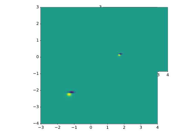
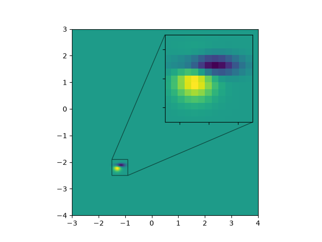
text_labels_and_annotations/accented_text
=============
Source
r"""
=============
Accented text
=============
Matplotlib supports accented characters via TeX mathtext or Unicode.
Using mathtext, the following accents are provided: \\hat, \\breve, \\grave,
\\bar, \\acute, \\tilde, \\vec, \\dot, \\ddot. All of them have the same
syntax, e.g. \\bar{o} yields "o overbar", \\ddot{o} yields "o umlaut".
Shortcuts such as \\"o \\'e \\`e \\~n \\.x \\^y are also supported.
"""
import matplotlib.pyplot as plt
# Mathtext demo
fig, ax = plt.subplots()
ax.plot(range(10))
ax.set_title(r'$\ddot{o}\acute{e}\grave{e}\hat{O}'
r'\breve{i}\bar{A}\tilde{n}\vec{q}$', fontsize=20)
# Shorthand is also supported and curly braces are optional
ax.set_xlabel(r"""$\"o\ddot o \'e\`e\~n\.x\^y$""", fontsize=20)
ax.text(4, 0.5, r"$F=m\ddot{x}$")
fig.tight_layout()
# %%
# You can also use Unicode characters directly in strings.
fig, ax = plt.subplots()
ax.set_title("GISCARD CHAHUTÉ À L'ASSEMBLÉE")
ax.set_xlabel("LE COUP DE DÉ DE DE GAULLE")
ax.set_ylabel('André was here!')
ax.text(0.2, 0.8, 'Institut für Festkörperphysik', rotation=45)
ax.text(0.4, 0.2, 'AVA (check kerning)')
plt.show()
text_labels_and_annotations/angle_annotation
===========================
Source
"""
===========================
Scale invariant angle label
===========================
This example shows how to create a scale invariant angle annotation. It is
often useful to mark angles between lines or inside shapes with a circular arc.
While Matplotlib provides an `~.patches.Arc`, an inherent problem when directly
using it for such purposes is that an arc being circular in data space is not
necessarily circular in display space. Also, the arc's radius is often best
defined in a coordinate system which is independent of the actual data
coordinates - at least if you want to be able to freely zoom into your plot
without the annotation growing to infinity.
This calls for a solution where the arc's center is defined in data space, but
its radius in a physical unit like points or pixels, or as a ratio of the Axes
dimension. The following ``AngleAnnotation`` class provides such solution.
The example below serves two purposes:
* It provides a ready-to-use solution for the problem of easily drawing angles
in graphs.
* It shows how to subclass a Matplotlib artist to enhance its functionality, as
well as giving a hands-on example on how to use Matplotlib's :ref:`transform
system <transforms_tutorial>`.
If mainly interested in the former, you may copy the below class and jump to
the :ref:`angle-annotation-usage` section.
"""
# %%
# AngleAnnotation class
# ---------------------
# The essential idea here is to subclass `~.patches.Arc` and set its transform
# to the `~.transforms.IdentityTransform`, making the parameters of the arc
# defined in pixel space.
# We then override the ``Arc``'s attributes ``_center``, ``theta1``,
# ``theta2``, ``width`` and ``height`` and make them properties, coupling to
# internal methods that calculate the respective parameters each time the
# attribute is accessed and thereby ensuring that the arc in pixel space stays
# synchronized with the input points and size.
# For example, each time the arc's drawing method would query its ``_center``
# attribute, instead of receiving the same number all over again, it will
# instead receive the result of the ``get_center_in_pixels`` method we defined
# in the subclass. This method transforms the center in data coordinates to
# pixels via the Axes transform ``ax.transData``. The size and the angles are
# calculated in a similar fashion, such that the arc changes its shape
# automatically when e.g. zooming or panning interactively.
#
# The functionality of this class allows to annotate the arc with a text. This
# text is a `~.text.Annotation` stored in an attribute ``text``. Since the
# arc's position and radius are defined only at draw time, we need to update
# the text's position accordingly. This is done by reimplementing the ``Arc``'s
# ``draw()`` method to let it call an updating method for the text.
#
# The arc and the text will be added to the provided Axes at instantiation: it
# is hence not strictly necessary to keep a reference to it.
import matplotlib.pyplot as plt
import numpy as np
from matplotlib.patches import Arc
from matplotlib.transforms import Bbox, IdentityTransform, TransformedBbox
class AngleAnnotation(Arc):
"""
Draws an arc between two vectors which appears circular in display space.
"""
def __init__(self, xy, p1, p2, size=75, unit="points", ax=None,
text="", textposition="inside", text_kw=None, **kwargs):
"""
Parameters
----------
xy, p1, p2 : tuple or array of two floats
Center position and two points. Angle annotation is drawn between
the two vectors connecting *p1* and *p2* with *xy*, respectively.
Units are data coordinates.
size : float
Diameter of the angle annotation in units specified by *unit*.
unit : str
One of the following strings to specify the unit of *size*:
* "pixels": pixels
* "points": points, use points instead of pixels to not have a
dependence on the DPI
* "axes width", "axes height": relative units of Axes width, height
* "axes min", "axes max": minimum or maximum of relative Axes
width, height
ax : `matplotlib.axes.Axes`, default: current Axes
The Axes to add the angle annotation to.
text : str
The text to mark the angle with.
textposition : {"inside", "outside", "edge"}
Whether to show the text in- or outside the arc. "edge" can be used
for custom positions anchored at the arc's edge.
text_kw : dict
Dictionary of arguments passed to the Annotation.
**kwargs
Further parameters are passed to `matplotlib.patches.Arc`. Use this
to specify, color, linewidth etc. of the arc.
"""
self.ax = ax or plt.gca()
self._xydata = xy # in data coordinates
self.vec1 = p1
self.vec2 = p2
self.size = size
self.unit = unit
self.textposition = textposition
super().__init__(self._xydata, size, size, angle=0.0,
theta1=self.theta1, theta2=self.theta2, **kwargs)
self.set_transform(IdentityTransform())
self.ax.add_patch(self)
self.kw = dict(ha="center", va="center",
xycoords=IdentityTransform(),
xytext=(0, 0), textcoords="offset points",
annotation_clip=True)
self.kw.update(text_kw or {})
self.text = self.ax.annotate(text, xy=self._center, **self.kw)
def get_size(self):
factor = 1.
if self.unit == "points":
factor = self.ax.figure.dpi / 72.
elif self.unit[:4] == "axes":
b = TransformedBbox(Bbox.unit(), self.ax.transAxes)
dic = {"max": max(b.width, b.height),
"min": min(b.width, b.height),
"width": b.width, "height": b.height}
factor = dic[self.unit[5:]]
return self.size * factor
def set_size(self, size):
self.size = size
def get_center_in_pixels(self):
"""return center in pixels"""
return self.ax.transData.transform(self._xydata)
def set_center(self, xy):
"""set center in data coordinates"""
self._xydata = xy
def get_theta(self, vec):
vec_in_pixels = self.ax.transData.transform(vec) - self._center
return np.rad2deg(np.arctan2(vec_in_pixels[1], vec_in_pixels[0]))
def get_theta1(self):
return self.get_theta(self.vec1)
def get_theta2(self):
return self.get_theta(self.vec2)
def set_theta(self, angle):
pass
# Redefine attributes of the Arc to always give values in pixel space
_center = property(get_center_in_pixels, set_center)
theta1 = property(get_theta1, set_theta)
theta2 = property(get_theta2, set_theta)
width = property(get_size, set_size)
height = property(get_size, set_size)
# The following two methods are needed to update the text position.
def draw(self, renderer):
self.update_text()
super().draw(renderer)
def update_text(self):
c = self._center
s = self.get_size()
angle_span = (self.theta2 - self.theta1) % 360
angle = np.deg2rad(self.theta1 + angle_span / 2)
r = s / 2
if self.textposition == "inside":
r = s / np.interp(angle_span, [60, 90, 135, 180],
[3.3, 3.5, 3.8, 4])
self.text.xy = c + r * np.array([np.cos(angle), np.sin(angle)])
if self.textposition == "outside":
def R90(a, r, w, h):
if a < np.arctan(h/2/(r+w/2)):
return np.sqrt((r+w/2)**2 + (np.tan(a)*(r+w/2))**2)
else:
c = np.sqrt((w/2)**2+(h/2)**2)
T = np.arcsin(c * np.cos(np.pi/2 - a + np.arcsin(h/2/c))/r)
xy = r * np.array([np.cos(a + T), np.sin(a + T)])
xy += np.array([w/2, h/2])
return np.sqrt(np.sum(xy**2))
def R(a, r, w, h):
aa = (a % (np.pi/4))*((a % (np.pi/2)) <= np.pi/4) + \
(np.pi/4 - (a % (np.pi/4)))*((a % (np.pi/2)) >= np.pi/4)
return R90(aa, r, *[w, h][::int(np.sign(np.cos(2*a)))])
bbox = self.text.get_window_extent()
X = R(angle, r, bbox.width, bbox.height)
trans = self.ax.figure.dpi_scale_trans.inverted()
offs = trans.transform(((X-s/2), 0))[0] * 72
self.text.set_position([offs*np.cos(angle), offs*np.sin(angle)])
# %%
# .. _angle-annotation-usage:
#
# Usage
# -----
#
# Required arguments to ``AngleAnnotation`` are the center of the arc, *xy*,
# and two points, such that the arc spans between the two vectors connecting
# *p1* and *p2* with *xy*, respectively. Those are given in data coordinates.
# Further arguments are the *size* of the arc and its *unit*. Additionally, a
# *text* can be specified, that will be drawn either in- or outside of the arc,
# according to the value of *textposition*. Usage of those arguments is shown
# below.
fig, ax = plt.subplots()
fig.canvas.draw() # Need to draw the figure to define renderer
ax.set_title("AngleLabel example")
# Plot two crossing lines and label each angle between them with the above
# ``AngleAnnotation`` tool.
center = (4.5, 650)
p1 = [(2.5, 710), (6.0, 605)]
p2 = [(3.0, 275), (5.5, 900)]
line1, = ax.plot(*zip(*p1))
line2, = ax.plot(*zip(*p2))
point, = ax.plot(*center, marker="o")
am1 = AngleAnnotation(center, p1[1], p2[1], ax=ax, size=75, text=r"$\alpha$")
am2 = AngleAnnotation(center, p2[1], p1[0], ax=ax, size=35, text=r"$\beta$")
am3 = AngleAnnotation(center, p1[0], p2[0], ax=ax, size=75, text=r"$\gamma$")
am4 = AngleAnnotation(center, p2[0], p1[1], ax=ax, size=35, text=r"$\theta$")
# Showcase some styling options for the angle arc, as well as the text.
p = [(6.0, 400), (5.3, 410), (5.6, 300)]
ax.plot(*zip(*p))
am5 = AngleAnnotation(p[1], p[0], p[2], ax=ax, size=40, text=r"$\Phi$",
linestyle="--", color="gray", textposition="outside",
text_kw=dict(fontsize=16, color="gray"))
# %%
# ``AngleLabel`` options
# ----------------------
#
# The *textposition* and *unit* keyword arguments may be used to modify the
# location of the text label, as shown below:
# Helper function to draw angle easily.
def plot_angle(ax, pos, angle, length=0.95, acol="C0", **kwargs):
vec2 = np.array([np.cos(np.deg2rad(angle)), np.sin(np.deg2rad(angle))])
xy = np.c_[[length, 0], [0, 0], vec2*length].T + np.array(pos)
ax.plot(*xy.T, color=acol)
return AngleAnnotation(pos, xy[0], xy[2], ax=ax, **kwargs)
fig, (ax1, ax2) = plt.subplots(nrows=2, sharex=True)
fig.suptitle("AngleLabel keyword arguments")
fig.canvas.draw() # Need to draw the figure to define renderer
# Showcase different text positions.
ax1.margins(y=0.4)
ax1.set_title("textposition")
kw = dict(size=75, unit="points", text=r"$60°$")
am6 = plot_angle(ax1, (2.0, 0), 60, textposition="inside", **kw)
am7 = plot_angle(ax1, (3.5, 0), 60, textposition="outside", **kw)
am8 = plot_angle(ax1, (5.0, 0), 60, textposition="edge",
text_kw=dict(bbox=dict(boxstyle="round", fc="w")), **kw)
am9 = plot_angle(ax1, (6.5, 0), 60, textposition="edge",
text_kw=dict(xytext=(30, 20), arrowprops=dict(arrowstyle="->",
connectionstyle="arc3,rad=-0.2")), **kw)
for x, text in zip([2.0, 3.5, 5.0, 6.5], ['"inside"', '"outside"', '"edge"',
'"edge", custom arrow']):
ax1.annotate(text, xy=(x, 0), xycoords=ax1.get_xaxis_transform(),
bbox=dict(boxstyle="round", fc="w"), ha="left", fontsize=8,
annotation_clip=True)
# Showcase different size units. The effect of this can best be observed
# by interactively changing the figure size
ax2.margins(y=0.4)
ax2.set_title("unit")
kw = dict(text=r"$60°$", textposition="outside")
am10 = plot_angle(ax2, (2.0, 0), 60, size=50, unit="pixels", **kw)
am11 = plot_angle(ax2, (3.5, 0), 60, size=50, unit="points", **kw)
am12 = plot_angle(ax2, (5.0, 0), 60, size=0.25, unit="axes min", **kw)
am13 = plot_angle(ax2, (6.5, 0), 60, size=0.25, unit="axes max", **kw)
for x, text in zip([2.0, 3.5, 5.0, 6.5], ['"pixels"', '"points"',
'"axes min"', '"axes max"']):
ax2.annotate(text, xy=(x, 0), xycoords=ax2.get_xaxis_transform(),
bbox=dict(boxstyle="round", fc="w"), ha="left", fontsize=8,
annotation_clip=True)
plt.show()
# %%
#
# .. admonition:: References
#
# The use of the following functions, methods, classes and modules is shown
# in this example:
#
# - `matplotlib.patches.Arc`
# - `matplotlib.axes.Axes.annotate` / `matplotlib.pyplot.annotate`
# - `matplotlib.text.Annotation`
# - `matplotlib.transforms.IdentityTransform`
# - `matplotlib.transforms.TransformedBbox`
# - `matplotlib.transforms.Bbox`
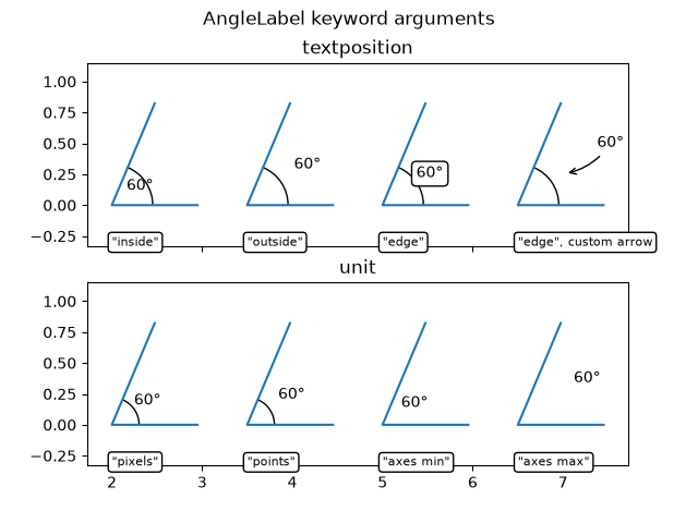
text_labels_and_annotations/angles_on_bracket_arrows
===================================
Source
"""
===================================
Angle annotations on bracket arrows
===================================
This example shows how to add angle annotations to bracket arrow styles
created using `.FancyArrowPatch`. *angleA* and *angleB* are measured from a
vertical line as positive (to the left) or negative (to the right). Blue
`.FancyArrowPatch` arrows indicate the directions of *angleA* and *angleB*
from the vertical and axes text annotate the angle sizes.
"""
import matplotlib.pyplot as plt
import numpy as np
from matplotlib.patches import FancyArrowPatch
def get_point_of_rotated_vertical(origin, line_length, degrees):
"""Return xy coordinates of the vertical line end rotated by degrees."""
rad = np.deg2rad(-degrees)
return [origin[0] + line_length * np.sin(rad),
origin[1] + line_length * np.cos(rad)]
fig, ax = plt.subplots()
ax.set(xlim=(0, 6), ylim=(-1, 5))
ax.set_title("Orientation of the bracket arrows relative to angleA and angleB")
style = ']-['
for i, angle in enumerate([-40, 0, 60]):
y = 2*i
arrow_centers = ((1, y), (5, y))
vlines = ((1, y + 0.5), (5, y + 0.5))
anglesAB = (angle, -angle)
bracketstyle = f"{style}, angleA={anglesAB[0]}, angleB={anglesAB[1]}"
bracket = FancyArrowPatch(*arrow_centers, arrowstyle=bracketstyle,
mutation_scale=42)
ax.add_patch(bracket)
ax.text(3, y + 0.05, bracketstyle, ha="center", va="bottom", fontsize=14)
ax.vlines([line[0] for line in vlines], [y, y], [line[1] for line in vlines],
linestyles="--", color="C0")
# Get the top coordinates for the drawn patches at A and B
patch_tops = [get_point_of_rotated_vertical(center, 0.5, angle)
for center, angle in zip(arrow_centers, anglesAB)]
# Define the connection directions for the annotation arrows
connection_dirs = (1, -1) if angle > 0 else (-1, 1)
# Add arrows and annotation text
arrowstyle = "Simple, tail_width=0.5, head_width=4, head_length=8"
for vline, dir, patch_top, angle in zip(vlines, connection_dirs,
patch_tops, anglesAB):
kw = dict(connectionstyle=f"arc3,rad={dir * 0.5}",
arrowstyle=arrowstyle, color="C0")
ax.add_patch(FancyArrowPatch(vline, patch_top, **kw))
ax.text(vline[0] - dir * 0.15, y + 0.7, f'{angle}°', ha="center",
va="center")
plt.show()
# %%
#
# .. admonition:: References
#
# The use of the following functions, methods, classes and modules is shown
# in this example:
#
# - `matplotlib.patches.ArrowStyle`
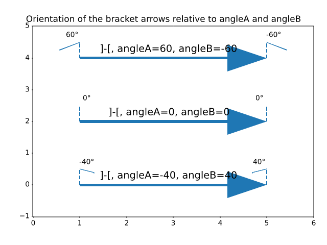
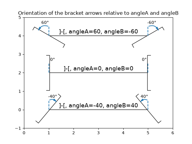
text_labels_and_annotations/annotation_basic
=================
Source
"""
=================
Annotating a plot
=================
This example shows how to annotate a plot with an arrow pointing to provided
coordinates. We modify the defaults of the arrow, to "shrink" it.
For a complete overview of the annotation capabilities, also see the
:ref:`annotation tutorial<annotations>`.
.. redirect-from:: /gallery/pyplots/annotation_basic
"""
import matplotlib.pyplot as plt
import numpy as np
fig, ax = plt.subplots()
t = np.arange(0.0, 5.0, 0.01)
s = np.cos(2*np.pi*t)
line, = ax.plot(t, s, lw=2)
ax.annotate('local max', xy=(2, 1), xytext=(3, 1.5),
arrowprops=dict(facecolor='black', shrink=0.05),
)
ax.set_ylim(-2, 2)
plt.show()
# %%
#
# .. admonition:: References
#
# The use of the following functions, methods, classes and modules is shown
# in this example:
#
# - `matplotlib.axes.Axes.annotate` / `matplotlib.pyplot.annotate`
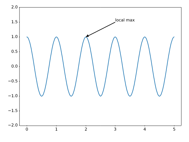
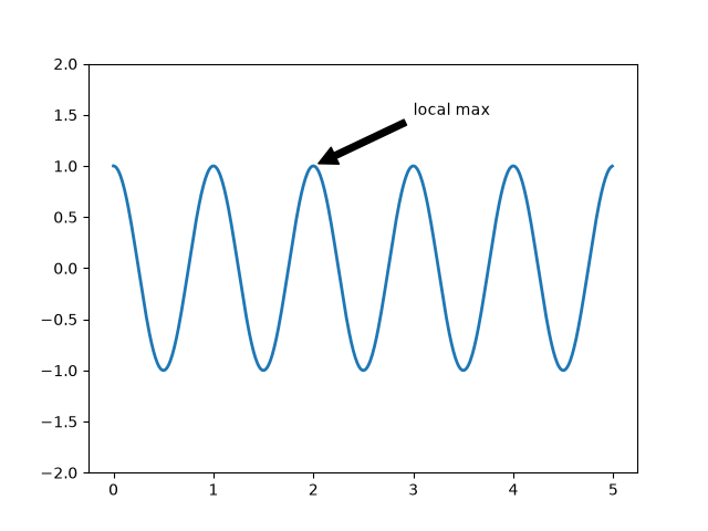
text_labels_and_annotations/annotation_demo
==============
Source
"""
==============
Annotate plots
==============
The following examples show ways to annotate plots in Matplotlib.
This includes highlighting specific points of interest and using various
visual tools to call attention to this point. For a more complete and in-depth
description of the annotation and text tools in Matplotlib, see the
:ref:`tutorial on annotation <annotations>`.
"""
import matplotlib.pyplot as plt
import numpy as np
from matplotlib.patches import Ellipse
from matplotlib.text import OffsetFrom
# %%
# Specifying text points and annotation points
# --------------------------------------------
#
# You must specify an annotation point ``xy=(x, y)`` to annotate this point.
# Additionally, you may specify a text point ``xytext=(x, y)`` for the location
# of the text for this annotation. Optionally, you can specify the coordinate
# system of *xy* and *xytext* with one of the following strings for *xycoords*
# and *textcoords* (default is 'data')::
#
# 'figure points' : points from the lower left corner of the figure
# 'figure pixels' : pixels from the lower left corner of the figure
# 'figure fraction' : (0, 0) is lower left of figure and (1, 1) is upper right
# 'axes points' : points from lower left corner of the Axes
# 'axes pixels' : pixels from lower left corner of the Axes
# 'axes fraction' : (0, 0) is lower left of Axes and (1, 1) is upper right
# 'offset points' : Specify an offset (in points) from the xy value
# 'offset pixels' : Specify an offset (in pixels) from the xy value
# 'data' : use the Axes data coordinate system
#
# Note: for physical coordinate systems (points or pixels) the origin is the
# (bottom, left) of the figure or Axes.
#
# Optionally, you can specify arrow properties which draws and arrow
# from the text to the annotated point by giving a dictionary of arrow
# properties
#
# Valid keys are::
#
# width : the width of the arrow in points
# frac : the fraction of the arrow length occupied by the head
# headwidth : the width of the base of the arrow head in points
# shrink : move the tip and base some percent away from the
# annotated point and text
# any key for matplotlib.patches.polygon (e.g., facecolor)
# Create our figure and data we'll use for plotting
fig, ax = plt.subplots(figsize=(4, 4))
t = np.arange(0.0, 5.0, 0.01)
s = np.cos(2*np.pi*t)
# Plot a line and add some simple annotations
line, = ax.plot(t, s)
ax.annotate('figure pixels',
xy=(10, 10), xycoords='figure pixels')
ax.annotate('figure points',
xy=(107, 110), xycoords='figure points',
fontsize=12)
ax.annotate('figure fraction',
xy=(.025, .975), xycoords='figure fraction',
horizontalalignment='left', verticalalignment='top',
fontsize=20)
# The following examples show off how these arrows are drawn.
ax.annotate('point offset from data',
xy=(3, 1), xycoords='data',
xytext=(-10, 90), textcoords='offset points',
arrowprops=dict(facecolor='black', shrink=0.05),
horizontalalignment='center', verticalalignment='bottom')
ax.annotate('axes fraction',
xy=(2, 1), xycoords='data',
xytext=(0.36, 0.68), textcoords='axes fraction',
arrowprops=dict(facecolor='black', shrink=0.05),
horizontalalignment='right', verticalalignment='top')
# You may also use negative points or pixels to specify from (right, top).
# E.g., (-10, 10) is 10 points to the left of the right side of the Axes and 10
# points above the bottom
ax.annotate('pixel offset from axes fraction',
xy=(1, 0), xycoords='axes fraction',
xytext=(-20, 20), textcoords='offset pixels',
horizontalalignment='right',
verticalalignment='bottom')
ax.set(xlim=(-1, 5), ylim=(-3, 5))
# %%
# Using multiple coordinate systems and axis types
# ------------------------------------------------
#
# You can specify the *xypoint* and the *xytext* in different positions and
# coordinate systems, and optionally turn on a connecting line and mark the
# point with a marker. Annotations work on polar Axes too.
#
# In the example below, the *xy* point is in native coordinates (*xycoords*
# defaults to 'data'). For a polar Axes, this is in (theta, radius) space.
# The text in the example is placed in the fractional figure coordinate system.
# Text keyword arguments like horizontal and vertical alignment are respected.
fig, ax = plt.subplots(subplot_kw=dict(projection='polar'), figsize=(3, 3))
r = np.arange(0, 1, 0.001)
theta = 2*2*np.pi*r
line, = ax.plot(theta, r)
ind = 800
thisr, thistheta = r[ind], theta[ind]
ax.plot([thistheta], [thisr], 'o')
ax.annotate('a polar annotation',
xy=(thistheta, thisr), # theta, radius
xytext=(0.05, 0.05), # fraction, fraction
textcoords='figure fraction',
arrowprops=dict(facecolor='black', shrink=0.05),
horizontalalignment='left',
verticalalignment='bottom')
# %%
# You can also use polar notation on a cartesian Axes. Here the native
# coordinate system ('data') is cartesian, so you need to specify the
# xycoords and textcoords as 'polar' if you want to use (theta, radius).
el = Ellipse((0, 0), 10, 20, facecolor='r', alpha=0.5)
fig, ax = plt.subplots(subplot_kw=dict(aspect='equal'))
ax.add_artist(el)
el.set_clip_box(ax.bbox)
ax.annotate('the top',
xy=(np.pi/2., 10.), # theta, radius
xytext=(np.pi/3, 20.), # theta, radius
xycoords='polar',
textcoords='polar',
arrowprops=dict(facecolor='black', shrink=0.05),
horizontalalignment='left',
verticalalignment='bottom',
clip_on=True) # clip to the Axes bounding box
ax.set(xlim=[-20, 20], ylim=[-20, 20])
# %%
# Customizing arrow and bubble styles
# -----------------------------------
#
# The arrow between *xytext* and the annotation point, as well as the bubble
# that covers the annotation text, are highly customizable. Below are a few
# parameter options as well as their resulting output.
fig, ax = plt.subplots(figsize=(8, 5))
t = np.arange(0.0, 5.0, 0.01)
s = np.cos(2*np.pi*t)
line, = ax.plot(t, s, lw=3)
ax.annotate(
'straight',
xy=(0, 1), xycoords='data',
xytext=(-50, 30), textcoords='offset points',
arrowprops=dict(arrowstyle="->"))
ax.annotate(
'arc3,\nrad 0.2',
xy=(0.5, -1), xycoords='data',
xytext=(-80, -60), textcoords='offset points',
arrowprops=dict(arrowstyle="->",
connectionstyle="arc3,rad=.2"))
ax.annotate(
'arc,\nangle 50',
xy=(1., 1), xycoords='data',
xytext=(-90, 50), textcoords='offset points',
arrowprops=dict(arrowstyle="->",
connectionstyle="arc,angleA=0,armA=50,rad=10"))
ax.annotate(
'arc,\narms',
xy=(1.5, -1), xycoords='data',
xytext=(-80, -60), textcoords='offset points',
arrowprops=dict(
arrowstyle="->",
connectionstyle="arc,angleA=0,armA=40,angleB=-90,armB=30,rad=7"))
ax.annotate(
'angle,\nangle 90',
xy=(2., 1), xycoords='data',
xytext=(-70, 30), textcoords='offset points',
arrowprops=dict(arrowstyle="->",
connectionstyle="angle,angleA=0,angleB=90,rad=10"))
ax.annotate(
'angle3,\nangle -90',
xy=(2.5, -1), xycoords='data',
xytext=(-80, -60), textcoords='offset points',
arrowprops=dict(arrowstyle="->",
connectionstyle="angle3,angleA=0,angleB=-90"))
ax.annotate(
'angle,\nround',
xy=(3., 1), xycoords='data',
xytext=(-60, 30), textcoords='offset points',
bbox=dict(boxstyle="round", fc="0.8"),
arrowprops=dict(arrowstyle="->",
connectionstyle="angle,angleA=0,angleB=90,rad=10"))
ax.annotate(
'angle,\nround4',
xy=(3.5, -1), xycoords='data',
xytext=(-70, -80), textcoords='offset points',
size=20,
bbox=dict(boxstyle="round4,pad=.5", fc="0.8"),
arrowprops=dict(arrowstyle="->",
connectionstyle="angle,angleA=0,angleB=-90,rad=10"))
ax.annotate(
'angle,\nshrink',
xy=(4., 1), xycoords='data',
xytext=(-60, 30), textcoords='offset points',
bbox=dict(boxstyle="round", fc="0.8"),
arrowprops=dict(arrowstyle="->",
shrinkA=0, shrinkB=10,
connectionstyle="angle,angleA=0,angleB=90,rad=10"))
# You can pass an empty string to get only annotation arrows rendered
ax.annotate('', xy=(4., 1.), xycoords='data',
xytext=(4.5, -1), textcoords='data',
arrowprops=dict(arrowstyle="<->",
connectionstyle="bar",
ec="k",
shrinkA=5, shrinkB=5))
ax.set(xlim=(-1, 5), ylim=(-4, 3))
# %%
# We'll create another figure so that it doesn't get too cluttered
fig, ax = plt.subplots()
el = Ellipse((2, -1), 0.5, 0.5)
ax.add_patch(el)
ax.annotate('$->$',
xy=(2., -1), xycoords='data',
xytext=(-150, -140), textcoords='offset points',
bbox=dict(boxstyle="round", fc="0.8"),
arrowprops=dict(arrowstyle="->",
patchB=el,
connectionstyle="angle,angleA=90,angleB=0,rad=10"))
ax.annotate('arrow\nfancy',
xy=(2., -1), xycoords='data',
xytext=(-100, 60), textcoords='offset points',
size=20,
arrowprops=dict(arrowstyle="fancy",
fc="0.6", ec="none",
patchB=el,
connectionstyle="angle3,angleA=0,angleB=-90"))
ax.annotate('arrow\nsimple',
xy=(2., -1), xycoords='data',
xytext=(100, 60), textcoords='offset points',
size=20,
arrowprops=dict(arrowstyle="simple",
fc="0.6", ec="none",
patchB=el,
connectionstyle="arc3,rad=0.3"))
ax.annotate('wedge',
xy=(2., -1), xycoords='data',
xytext=(-100, -100), textcoords='offset points',
size=20,
arrowprops=dict(arrowstyle="wedge,tail_width=0.7",
fc="0.6", ec="none",
patchB=el,
connectionstyle="arc3,rad=-0.3"))
ax.annotate('bubble,\ncontours',
xy=(2., -1), xycoords='data',
xytext=(0, -70), textcoords='offset points',
size=20,
bbox=dict(boxstyle="round",
fc=(1.0, 0.7, 0.7),
ec=(1., .5, .5)),
arrowprops=dict(arrowstyle="wedge,tail_width=1.",
fc=(1.0, 0.7, 0.7), ec=(1., .5, .5),
patchA=None,
patchB=el,
relpos=(0.2, 0.8),
connectionstyle="arc3,rad=-0.1"))
ax.annotate('bubble',
xy=(2., -1), xycoords='data',
xytext=(55, 0), textcoords='offset points',
size=20, va="center",
bbox=dict(boxstyle="round", fc=(1.0, 0.7, 0.7), ec="none"),
arrowprops=dict(arrowstyle="wedge,tail_width=1.",
fc=(1.0, 0.7, 0.7), ec="none",
patchA=None,
patchB=el,
relpos=(0.2, 0.5)))
ax.set(xlim=(-1, 5), ylim=(-5, 3))
# %%
# More examples of coordinate systems
# -----------------------------------
#
# Below we'll show a few more examples of coordinate systems and how the
# location of annotations may be specified.
fig, (ax1, ax2) = plt.subplots(1, 2)
bbox_args = dict(boxstyle="round", fc="0.8")
arrow_args = dict(arrowstyle="->")
# Here we'll demonstrate the extents of the coordinate system and how
# we place annotating text.
ax1.annotate('figure fraction : 0, 0', xy=(0, 0), xycoords='figure fraction',
xytext=(20, 20), textcoords='offset points',
ha="left", va="bottom",
bbox=bbox_args,
arrowprops=arrow_args)
ax1.annotate('figure fraction : 1, 1', xy=(1, 1), xycoords='figure fraction',
xytext=(-20, -20), textcoords='offset points',
ha="right", va="top",
bbox=bbox_args,
arrowprops=arrow_args)
ax1.annotate('axes fraction : 0, 0', xy=(0, 0), xycoords='axes fraction',
xytext=(20, 20), textcoords='offset points',
ha="left", va="bottom",
bbox=bbox_args,
arrowprops=arrow_args)
ax1.annotate('axes fraction : 1, 1', xy=(1, 1), xycoords='axes fraction',
xytext=(-20, -20), textcoords='offset points',
ha="right", va="top",
bbox=bbox_args,
arrowprops=arrow_args)
# It is also possible to generate draggable annotations
an1 = ax1.annotate('Drag me 1', xy=(.5, .7), xycoords='data',
ha="center", va="center",
bbox=bbox_args)
an2 = ax1.annotate('Drag me 2', xy=(.5, .5), xycoords=an1,
xytext=(.5, .3), textcoords='axes fraction',
ha="center", va="center",
bbox=bbox_args,
arrowprops=dict(patchB=an1.get_bbox_patch(),
connectionstyle="arc3,rad=0.2",
**arrow_args))
an1.draggable()
an2.draggable()
an3 = ax1.annotate('', xy=(.5, .5), xycoords=an2,
xytext=(.5, .5), textcoords=an1,
ha="center", va="center",
bbox=bbox_args,
arrowprops=dict(patchA=an1.get_bbox_patch(),
patchB=an2.get_bbox_patch(),
connectionstyle="arc3,rad=0.2",
**arrow_args))
# Finally we'll show off some more complex annotation and placement
text = ax2.annotate('xy=(0, 1)\nxycoords=("data", "axes fraction")',
xy=(0, 1), xycoords=("data", 'axes fraction'),
xytext=(0, -20), textcoords='offset points',
ha="center", va="top",
bbox=bbox_args,
arrowprops=arrow_args)
ax2.annotate('xy=(0.5, 0)\nxycoords=artist',
xy=(0.5, 0.), xycoords=text,
xytext=(0, -20), textcoords='offset points',
ha="center", va="top",
bbox=bbox_args,
arrowprops=arrow_args)
ax2.annotate('xy=(0.8, 0.5)\nxycoords=ax1.transData',
xy=(0.8, 0.5), xycoords=ax1.transData,
xytext=(10, 10),
textcoords=OffsetFrom(ax2.bbox, (0, 0), "points"),
ha="left", va="bottom",
bbox=bbox_args,
arrowprops=arrow_args)
ax2.set(xlim=[-2, 2], ylim=[-2, 2])
plt.show()
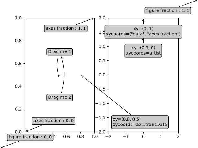
text_labels_and_annotations/annotation_polar
====================
Source
"""
====================
Annotate polar plots
====================
This example shows how to create an annotation on a polar graph.
For a complete overview of the annotation capabilities, also see the
:ref:`annotations`.
.. redirect-from:: /gallery/pyplots/annotation_polar
"""
import matplotlib.pyplot as plt
import numpy as np
fig = plt.figure()
ax = fig.add_subplot(projection='polar')
r = np.arange(0, 1, 0.001)
theta = 2 * 2*np.pi * r
line, = ax.plot(theta, r, color='#ee8d18', lw=3)
ind = 800
thisr, thistheta = r[ind], theta[ind]
ax.plot([thistheta], [thisr], 'o')
ax.annotate('a polar annotation',
xy=(thistheta, thisr), # theta, radius
xytext=(0.05, 0.05), # fraction, fraction
textcoords='figure fraction',
arrowprops=dict(facecolor='black', shrink=0.05),
horizontalalignment='left',
verticalalignment='bottom',
)
plt.show()
# %%
#
# .. admonition:: References
#
# The use of the following functions, methods, classes and modules is shown
# in this example:
#
# - `matplotlib.projections.polar`
# - `matplotlib.axes.Axes.annotate` / `matplotlib.pyplot.annotate`
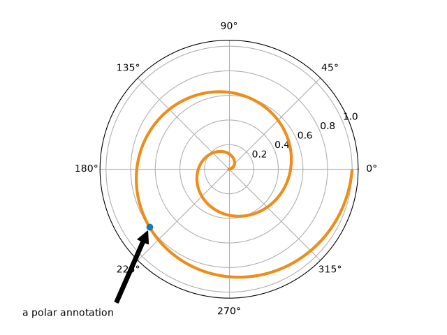
text_labels_and_annotations/arrow_demo
==========
Source
"""
==========
Arrow Demo
==========
Three ways of drawing arrows to encode arrow "strength" (e.g., transition
probabilities in a Markov model) using arrow length, width, or alpha (opacity).
"""
import itertools
import matplotlib.pyplot as plt
import numpy as np
def make_arrow_graph(ax, data, size=4, display='length', shape='right',
max_arrow_width=0.03, arrow_sep=0.02, alpha=0.5,
normalize_data=False, ec=None, labelcolor=None,
**kwargs):
"""
Makes an arrow plot.
Parameters
----------
ax
The Axes where the graph is drawn.
data
Dict with probabilities for the bases and pair transitions.
size
Size of the plot, in inches.
display : {'length', 'width', 'alpha'}
The arrow property to change.
shape : {'full', 'left', 'right'}
For full or half arrows.
max_arrow_width : float
Maximum width of an arrow, in data coordinates.
arrow_sep : float
Separation between arrows in a pair, in data coordinates.
alpha : float
Maximum opacity of arrows.
**kwargs
`.FancyArrow` properties, e.g. *linewidth* or *edgecolor*.
"""
ax.set(xlim=(-0.25, 1.25), ylim=(-0.25, 1.25), xticks=[], yticks=[],
title=f'flux encoded as arrow {display}')
max_text_size = size * 12
min_text_size = size
label_text_size = size * 4
bases = 'ATGC'
coords = {
'A': np.array([0, 1]),
'T': np.array([1, 1]),
'G': np.array([0, 0]),
'C': np.array([1, 0]),
}
colors = {'A': 'r', 'T': 'k', 'G': 'g', 'C': 'b'}
for base in bases:
fontsize = np.clip(max_text_size * data[base]**(1/2),
min_text_size, max_text_size)
ax.text(*coords[base], f'${base}_3$',
color=colors[base], size=fontsize,
horizontalalignment='center', verticalalignment='center',
weight='bold')
arrow_h_offset = 0.25 # data coordinates, empirically determined
max_arrow_length = 1 - 2 * arrow_h_offset
max_head_width = 2.5 * max_arrow_width
max_head_length = 2 * max_arrow_width
sf = 0.6 # max arrow size represents this in data coords
if normalize_data:
# find maximum value for rates, i.e. where keys are 2 chars long
max_val = max((v for k, v in data.items() if len(k) == 2), default=0)
# divide rates by max val, multiply by arrow scale factor
for k, v in data.items():
data[k] = v / max_val * sf
# iterate over strings 'AT', 'TA', 'AG', 'GA', etc.
for pair in map(''.join, itertools.permutations(bases, 2)):
# set the length of the arrow
if display == 'length':
length = (max_head_length
+ data[pair] / sf * (max_arrow_length - max_head_length))
else:
length = max_arrow_length
# set the transparency of the arrow
if display == 'alpha':
alpha = min(data[pair] / sf, alpha)
# set the width of the arrow
if display == 'width':
scale = data[pair] / sf
width = max_arrow_width * scale
head_width = max_head_width * scale
head_length = max_head_length * scale
else:
width = max_arrow_width
head_width = max_head_width
head_length = max_head_length
fc = colors[pair[0]]
cp0 = coords[pair[0]]
cp1 = coords[pair[1]]
# unit vector in arrow direction
delta = cos, sin = (cp1 - cp0) / np.hypot(*(cp1 - cp0))
x_pos, y_pos = (
(cp0 + cp1) / 2 # midpoint
- delta * length / 2 # half the arrow length
+ np.array([-sin, cos]) * arrow_sep # shift outwards by arrow_sep
)
ax.arrow(
x_pos, y_pos, cos * length, sin * length,
fc=fc, ec=ec or fc, alpha=alpha, width=width,
head_width=head_width, head_length=head_length, shape=shape,
length_includes_head=True,
**kwargs
)
# figure out coordinates for text:
# if drawing relative to base: x and y are same as for arrow
# dx and dy are one arrow width left and up
orig_positions = {
'base': [3 * max_arrow_width, 3 * max_arrow_width],
'center': [length / 2, 3 * max_arrow_width],
'tip': [length - 3 * max_arrow_width, 3 * max_arrow_width],
}
# for diagonal arrows, put the label at the arrow base
# for vertical or horizontal arrows, center the label
where = 'base' if (cp0 != cp1).all() else 'center'
# rotate based on direction of arrow (cos, sin)
M = [[cos, -sin], [sin, cos]]
x, y = np.dot(M, orig_positions[where]) + [x_pos, y_pos]
label = r'$r_{_{\mathrm{%s}}}$' % (pair,)
ax.text(x, y, label, size=label_text_size, ha='center', va='center',
color=labelcolor or fc)
if __name__ == '__main__':
data = { # test data
'A': 0.4, 'T': 0.3, 'G': 0.6, 'C': 0.2,
'AT': 0.4, 'AC': 0.3, 'AG': 0.2,
'TA': 0.2, 'TC': 0.3, 'TG': 0.4,
'CT': 0.2, 'CG': 0.3, 'CA': 0.2,
'GA': 0.1, 'GT': 0.4, 'GC': 0.1,
}
size = 4
fig = plt.figure(figsize=(3 * size, size), layout="constrained")
axs = fig.subplot_mosaic([["length", "width", "alpha"]])
for display, ax in axs.items():
make_arrow_graph(
ax, data, display=display, linewidth=0.001, edgecolor=None,
normalize_data=True, size=size)
plt.show()
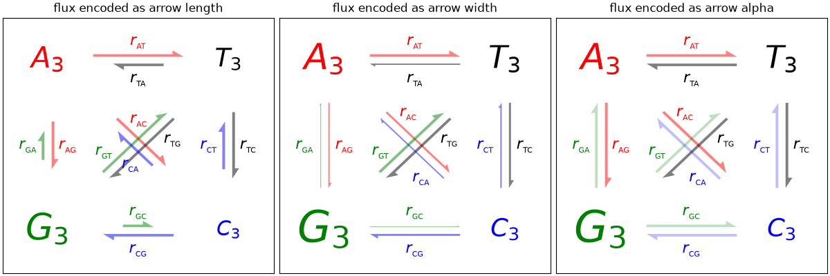
text_labels_and_annotations/autowrap
==============
Source
"""
==============
Auto-wrap text
==============
Matplotlib can wrap text automatically, but if it's too long, the text will
still be displayed slightly outside the boundaries of the axis.
Note: Auto-wrapping does not work together with
``savefig(..., bbox_inches='tight')``. The 'tight' setting rescales the canvas
to accommodate all content and happens before wrapping. This affects
``%matplotlib inline`` in IPython and Jupyter notebooks where the inline
setting uses ``bbox_inches='tight'`` by default when saving the image to
embed.
"""
import matplotlib.pyplot as plt
fig = plt.figure()
plt.axis((0, 10, 0, 10))
t = ("This is a really long string that I'd rather have wrapped so that it "
"doesn't go outside of the figure, but if it's long enough it will go "
"off the top or bottom!")
plt.text(4, 1, t, ha='left', rotation=15, wrap=True)
plt.text(6, 5, t, ha='left', rotation=15, wrap=True)
plt.text(5, 5, t, ha='right', rotation=-15, wrap=True)
plt.text(5, 10, t, fontsize=18, style='oblique', ha='center',
va='top', wrap=True)
plt.text(3, 4, t, family='serif', style='italic', ha='right', wrap=True)
plt.text(-1, 0, t, ha='left', rotation=-15, wrap=True)
plt.show()
text_labels_and_annotations/custom_legends
======================
Source
"""
======================
Compose custom legends
======================
Composing custom legends piece-by-piece.
.. note::
For more information on creating and customizing legends, see the following
pages:
* :ref:`legend_guide`
* :doc:`/gallery/text_labels_and_annotations/legend_demo`
Sometimes you don't want a legend that is explicitly tied to data that
you have plotted. For example, say you have plotted 10 lines, but don't
want a legend item to show up for each one. If you simply plot the lines
and call ``ax.legend()``, you will get the following:
"""
import matplotlib.pyplot as plt
import numpy as np
# sphinx_gallery_thumbnail_number = 2
import matplotlib as mpl
from matplotlib import cycler
# Fixing random state for reproducibility
np.random.seed(19680801)
# %%
N = 10
data = (np.geomspace(1, 10, 100) + np.random.randn(N, 100)).T
cmap = plt.colormaps["coolwarm"]
mpl.rcParams['axes.prop_cycle'] = cycler(color=cmap(np.linspace(0, 1, N)))
fig, ax = plt.subplots()
lines = ax.plot(data)
# %%
# Since the data does not have any labels, creating a legend requires
# us to define the icons and labels.
# In this case, we can compose a legend using Matplotlib objects that aren't
# explicitly tied to the data that was plotted. For example:
from matplotlib.lines import Line2D
custom_lines = [Line2D([0], [0], color=cmap(0.), lw=4),
Line2D([0], [0], color=cmap(.5), lw=4),
Line2D([0], [0], color=cmap(1.), lw=4)]
fig, ax = plt.subplots()
lines = ax.plot(data)
ax.legend(custom_lines, ['Cold', 'Medium', 'Hot'])
# %%
# There are many other Matplotlib objects that can be used in this way. In the
# code below we've listed a few common ones.
from matplotlib.lines import Line2D
from matplotlib.patches import Patch
legend_elements = [Line2D([0], [0], color='b', lw=4, label='Line'),
Line2D([0], [0], marker='o', color='w', label='Scatter',
markerfacecolor='g', markersize=15),
Patch(facecolor='orange', edgecolor='r',
label='Color Patch')]
# Create the figure
fig, ax = plt.subplots()
ax.legend(handles=legend_elements, loc='center')
plt.show()
text_labels_and_annotations/demo_annotation_box
======================
Source
"""
======================
Artists as annotations
======================
`.AnnotationBbox` facilitates using arbitrary artists as annotations, i.e. data at
position *xy* is annotated by a box containing an artist at position *xybox*. The
coordinate systems for these points are set via the *xycoords* and *boxcoords*
parameters, respectively; see the *xycoords* and *textcoords* parameters of
`.Axes.annotate` for a full listing of supported coordinate systems.
The box containing the artist is a subclass of `.OffsetBox`, which is a container
artist for positioning an artist relative to a parent artist.
"""
from pathlib import Path
import PIL
import matplotlib.pyplot as plt
import numpy as np
from matplotlib import get_data_path
from matplotlib.offsetbox import AnnotationBbox, DrawingArea, OffsetImage, TextArea
from matplotlib.patches import Annulus, Circle, ConnectionPatch
# %%%%
# Text
# ====
#
# `.AnnotationBbox` supports positioning annotations relative to data, Artists, and
# callables, as described in :ref:`annotations`. The `.TextArea` is used to create a
# textbox that is not explicitly attached to an axes, which allows it to be used for
# annotating figure objects. When annotating an axes element (such as a plot) with text,
# use `.Axes.annotate` because it will create the text artist for you.
fig, axd = plt.subplot_mosaic([['t1', '.', 't2']], layout='compressed')
# Define a 1st position to annotate (display it with a marker)
xy1 = (.25, .75)
xy2 = (.75, .25)
axd['t1'].plot(*xy1, ".r")
axd['t2'].plot(*xy2, ".r")
axd['t1'].set(xlim=(0, 1), ylim=(0, 1), aspect='equal')
axd['t2'].set(xlim=(0, 1), ylim=(0, 1), aspect='equal')
# Draw a connection patch arrow between the points
c = ConnectionPatch(xyA=xy1, xyB=xy2,
coordsA=axd['t1'].transData, coordsB=axd['t2'].transData,
arrowstyle='->')
fig.add_artist(c)
# Annotate the ConnectionPatch position ('Test 1')
offsetbox = TextArea("Test 1")
# place the annotation above the midpoint of c
ab1 = AnnotationBbox(offsetbox,
xy=(.5, .5),
xybox=(0, 30),
xycoords=c,
boxcoords="offset points",
arrowprops=dict(arrowstyle="->"),
bboxprops=dict(boxstyle="sawtooth"))
fig.add_artist(ab1)
# %%%%
# Images
# ======
# The `.OffsetImage` container facilitates using images as annotations
fig, ax = plt.subplots()
# Define a position to annotate
xy = (0.3, 0.55)
ax.scatter(*xy, s=200, marker='X')
# Annotate a position with an image generated from an array of pixels
arr = np.arange(100).reshape((10, 10))
im = OffsetImage(arr, zoom=2, cmap='viridis')
im.image.axes = ax
# place the image NW of xy
ab = AnnotationBbox(im, xy=xy,
xybox=(-50., 50.),
xycoords='data',
boxcoords="offset points",
pad=0.3,
arrowprops=dict(arrowstyle="->"))
ax.add_artist(ab)
# Annotate the position with an image from file (a Grace Hopper portrait)
img_fp = Path(get_data_path(), "sample_data", "grace_hopper.jpg")
with PIL.Image.open(img_fp) as arr_img:
imagebox = OffsetImage(arr_img, zoom=0.2)
imagebox.image.axes = ax
# place the image SE of xy
ab = AnnotationBbox(imagebox, xy=xy,
xybox=(120., -80.),
xycoords='data',
boxcoords="offset points",
pad=0.5,
arrowprops=dict(
arrowstyle="->",
connectionstyle="angle,angleA=0,angleB=90,rad=3")
)
ax.add_artist(ab)
# Fix the display limits to see everything
ax.set(xlim=(0, 1), ylim=(0, 1))
plt.show()
# %%%%
# Arbitrary Artists
# =================
#
# Multiple and arbitrary artists can be placed inside a `.DrawingArea`.
# make this the thumbnail image
# sphinx_gallery_thumbnail_number = 3
fig, ax = plt.subplots()
# Define a position to annotate
xy = (0.05, 0.5)
ax.scatter(*xy, s=500, marker='X')
# Annotate the position with a circle and annulus
da = DrawingArea(120, 120)
p = Circle((30, 30), 25, color='C0')
da.add_artist(p)
q = Annulus((65, 65), 50, 5, color='C1')
da.add_artist(q)
# Use the drawing area as an annotation
ab = AnnotationBbox(da, xy=xy,
xybox=(.55, xy[1]),
xycoords='data',
boxcoords=("axes fraction", "data"),
box_alignment=(0, 0.5),
arrowprops=dict(arrowstyle="->"),
bboxprops=dict(alpha=0.5))
ax.add_artist(ab)
# Fix the display limits to see everything
ax.set(xlim=(0, 1), ylim=(0, 1))
plt.show()
# %%
#
# .. admonition:: References
#
# The use of the following functions, methods, classes and modules is shown
# in this example:
#
# - `matplotlib.offsetbox.TextArea`
# - `matplotlib.offsetbox.DrawingArea`
# - `matplotlib.offsetbox.OffsetImage`
# - `matplotlib.offsetbox.AnnotationBbox`
#
# .. tags::
# component: annotation, styling: position
FileNotFoundError: [Errno 2] No such file or directory: '/home/runner/work/matplotvite/matplotvite/python/matplotvite/sample_data/grace_hopper.jpg'
text_labels_and_annotations/demo_text_path
======================
Source
"""
======================
Using a text as a Path
======================
`.TextPath` creates a `.Path` that is the outline of the characters of a text.
The resulting path can be employed e.g. as a clip path for an image.
"""
from PIL import Image
import matplotlib.pyplot as plt
import numpy as np
from matplotlib.cbook import get_sample_data
from matplotlib.image import BboxImage
from matplotlib.offsetbox import AnchoredOffsetbox, AnnotationBbox, AuxTransformBox
from matplotlib.patches import PathPatch, Shadow
from matplotlib.text import TextPath
from matplotlib.transforms import IdentityTransform
class PathClippedImagePatch(PathPatch):
"""
The given image is used to draw the face of the patch. Internally,
it uses BboxImage whose clippath set to the path of the patch.
FIXME : The result is currently dpi dependent.
"""
def __init__(self, path, bbox_image, **kwargs):
super().__init__(path, **kwargs)
self.bbox_image = BboxImage(
self.get_window_extent, norm=None, origin=None)
self.bbox_image.set_data(bbox_image)
def set_facecolor(self, color):
"""Simply ignore facecolor."""
super().set_facecolor("none")
def draw(self, renderer=None):
# the clip path must be updated every draw. any solution? -JJ
self.bbox_image.set_clip_path(self._path, self.get_transform())
self.bbox_image.draw(renderer)
super().draw(renderer)
if __name__ == "__main__":
fig, (ax1, ax2) = plt.subplots(2)
# EXAMPLE 1
arr = Image.open(get_sample_data("grace_hopper.jpg"))
text_path = TextPath((0, 0), "!?", size=150)
p = PathClippedImagePatch(text_path, arr, ec="k")
# make offset box
offsetbox = AuxTransformBox(IdentityTransform())
offsetbox.add_artist(p)
# make anchored offset box
ao = AnchoredOffsetbox(loc='upper left', child=offsetbox, frameon=True,
borderpad=0.2)
ax1.add_artist(ao)
# another text
for usetex, ypos, string in [
(False, 0.25, r"textpath supports mathtext"),
(True, 0.05, r"textpath supports \TeX"),
]:
text_path = TextPath((0, 0), string, size=20, usetex=usetex)
p1 = PathPatch(text_path, ec="w", lw=3, fc="w", alpha=0.9)
p2 = PathPatch(text_path, ec="none", fc="k")
offsetbox2 = AuxTransformBox(IdentityTransform())
offsetbox2.add_artist(p1)
offsetbox2.add_artist(p2)
ab = AnnotationBbox(offsetbox2, (0.95, ypos),
xycoords='axes fraction',
boxcoords="offset points",
box_alignment=(1., 0.),
frameon=False,
)
ax1.add_artist(ab)
ax1.imshow([[0, 1, 2], [1, 2, 3]], cmap="gist_gray_r",
interpolation="bilinear", aspect="auto")
# EXAMPLE 2
arr = np.arange(256).reshape(1, 256)
for usetex, xpos, string in [
(False, 0.25,
r"$\left[\sum_{n=1}^\infty\frac{-e^{i\pi}}{2^n}\right]$!"),
(True, 0.75,
r"$\displaystyle\left[\sum_{n=1}^\infty"
r"\frac{-e^{i\pi}}{2^n}\right]$!"),
]:
text_path = TextPath((0, 0), string, size=40, usetex=usetex)
text_patch = PathClippedImagePatch(text_path, arr, ec="none")
shadow1 = Shadow(text_patch, 1, -1, fc="none", ec="0.6", lw=3)
shadow2 = Shadow(text_patch, 1, -1, fc="0.3", ec="none")
# make offset box
offsetbox = AuxTransformBox(IdentityTransform())
offsetbox.add_artist(shadow1)
offsetbox.add_artist(shadow2)
offsetbox.add_artist(text_patch)
# place the anchored offset box using AnnotationBbox
ab = AnnotationBbox(offsetbox, (xpos, 0.5), box_alignment=(0.5, 0.5))
ax2.add_artist(ab)
ax2.set_xlim(0, 1)
ax2.set_ylim(0, 1)
plt.show()
RuntimeError: Failed to process string with tex because latex could not be found
text_labels_and_annotations/demo_text_rotation_mode
==================
Source
r"""
==================
Text rotation mode
==================
This example illustrates the effect of ``rotation_mode`` on the positioning
of rotated text.
Rotated `.Text`\s are created by passing the parameter ``rotation`` to
the constructor or the Axes' method `~.axes.Axes.text`.
The actual positioning depends on the additional parameters
``horizontalalignment``, ``verticalalignment`` and ``rotation_mode``.
``rotation_mode`` determines the order of rotation and alignment:
- ``rotation_mode='default'`` (or None) first rotates the text and then aligns
the bounding box of the rotated text.
- ``rotation_mode='anchor'`` aligns the unrotated text and then rotates the
text around the point of alignment.
.. redirect-from:: /gallery/text_labels_and_annotations/text_rotation
"""
import matplotlib.pyplot as plt
def test_rotation_mode(fig, mode):
ha_list = ["left", "center", "right"]
va_list = ["top", "center", "baseline", "bottom"]
axs = fig.subplots(len(va_list), len(ha_list), sharex=True, sharey=True,
subplot_kw=dict(aspect=1),
gridspec_kw=dict(hspace=0, wspace=0))
# labels and title
for ha, ax in zip(ha_list, axs[-1, :]):
ax.set_xlabel(ha)
for va, ax in zip(va_list, axs[:, 0]):
ax.set_ylabel(va)
axs[0, 1].set_title(f"rotation_mode='{mode}'", size="large")
kw = (
{} if mode == "default" else
{"bbox": dict(boxstyle="square,pad=0.", ec="none", fc="C1", alpha=0.3)}
)
texts = {}
# use a different text alignment in each Axes
for i, va in enumerate(va_list):
for j, ha in enumerate(ha_list):
ax = axs[i, j]
# prepare Axes layout
ax.set(xticks=[], yticks=[])
ax.axvline(0.5, color="skyblue", zorder=0)
ax.axhline(0.5, color="skyblue", zorder=0)
ax.plot(0.5, 0.5, color="C0", marker="o", zorder=1)
# add text with rotation and alignment settings
tx = ax.text(0.5, 0.5, "Tpg",
size="x-large", rotation=40,
horizontalalignment=ha, verticalalignment=va,
rotation_mode=mode, **kw)
texts[ax] = tx
if mode == "default":
# highlight bbox
fig.canvas.draw()
for ax, text in texts.items():
bb = text.get_window_extent().transformed(ax.transData.inverted())
rect = plt.Rectangle((bb.x0, bb.y0), bb.width, bb.height,
facecolor="C1", alpha=0.3, zorder=2)
ax.add_patch(rect)
fig = plt.figure(figsize=(8, 5))
subfigs = fig.subfigures(1, 2)
test_rotation_mode(subfigs[0], "default")
test_rotation_mode(subfigs[1], "anchor")
plt.show()
# %%
#
# .. admonition:: References
#
# The use of the following functions, methods, classes and modules is shown
# in this example:
#
# - `matplotlib.axes.Axes.text` / `matplotlib.pyplot.text`
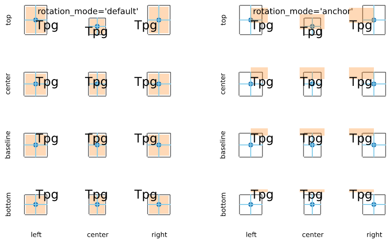
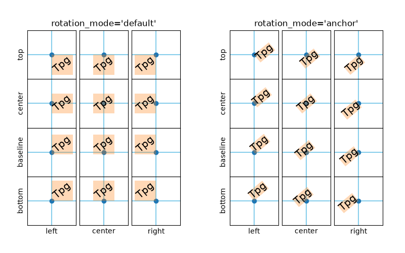
text_labels_and_annotations/dfrac_demo
=========================================
Source
r"""
=========================================
The difference between \\dfrac and \\frac
=========================================
In this example, the differences between the \\dfrac and \\frac TeX macros are
illustrated; in particular, the difference between display style and text style
fractions when using Mathtext.
.. versionadded:: 2.1
.. note::
To use \\dfrac with the LaTeX engine (text.usetex : True), you need to
import the amsmath package with :rc:`text.latex.preamble`, which is
an unsupported feature; therefore, it is probably a better idea to just
use the \\displaystyle option before the \\frac macro to get this behavior
with the LaTeX engine.
"""
import matplotlib.pyplot as plt
fig = plt.figure(figsize=(5.25, 0.75))
fig.text(0.5, 0.3, r'\dfrac: $\dfrac{a}{b}$',
horizontalalignment='center', verticalalignment='center')
fig.text(0.5, 0.7, r'\frac: $\frac{a}{b}$',
horizontalalignment='center', verticalalignment='center')
plt.show()


text_labels_and_annotations/fancyarrow_demo
================================
Source
"""
================================
Annotation arrow style reference
================================
Overview of the available `.ArrowStyle` settings. These are used for the *arrowstyle*
parameter of `~.Axes.annotate` and `.FancyArrowPatch`.
Each style can be configured with a set of parameters, which are stated along with
their default values.
"""
import inspect
import itertools
import re
import matplotlib.pyplot as plt
from matplotlib.patches import ArrowStyle
styles = ArrowStyle.get_styles()
ncol = 2
nrow = (len(styles) + 1) // ncol
gridspec_kw = dict(wspace=0, hspace=0.05, left=0, right=1, bottom=0, top=1)
fig, axs = plt.subplots(1 + nrow, ncol,
figsize=(4 * ncol, 1 + nrow), gridspec_kw=gridspec_kw)
for ax in axs.flat:
ax.set_xlim(-0.1, 4)
ax.set_axis_off()
for ax in axs[0, :]:
ax.text(0, 0.5, "arrowstyle", size="large", color="tab:blue")
ax.text(1.4, .5, "default parameters", size="large")
for ax, (stylename, stylecls) in zip(axs[1:, :].T.flat, styles.items()):
# draw dot and annotation with arrowstyle
l, = ax.plot(1.25, 0, "o", color="darkgrey")
ax.annotate(stylename, (1.25, 0), (0, 0),
size="large", color="tab:blue", va="center", family="monospace",
arrowprops=dict(
arrowstyle=stylename, connectionstyle="arc3,rad=0",
color="black", shrinkA=5, shrinkB=5, patchB=l,
),
bbox=dict(boxstyle="square", fc="w", ec="darkgrey"))
# draw default parameters
# wrap at every nth comma (n = 1 or 2, depending on text length)
s = str(inspect.signature(stylecls))[1:-1]
n = 2 if s.count(',') > 3 else 1
ax.text(1.4, 0,
re.sub(', ', lambda m, c=itertools.count(1): m.group()
if next(c) % n else '\n', s),
verticalalignment="center", color="0.3")
plt.show()
# %%
#
# .. admonition:: References
#
# The use of the following functions, methods, classes and modules is shown
# in this example:
#
# - `matplotlib.patches`
# - `matplotlib.patches.ArrowStyle`
# - ``matplotlib.patches.ArrowStyle.get_styles``
# - `matplotlib.axes.Axes.annotate`
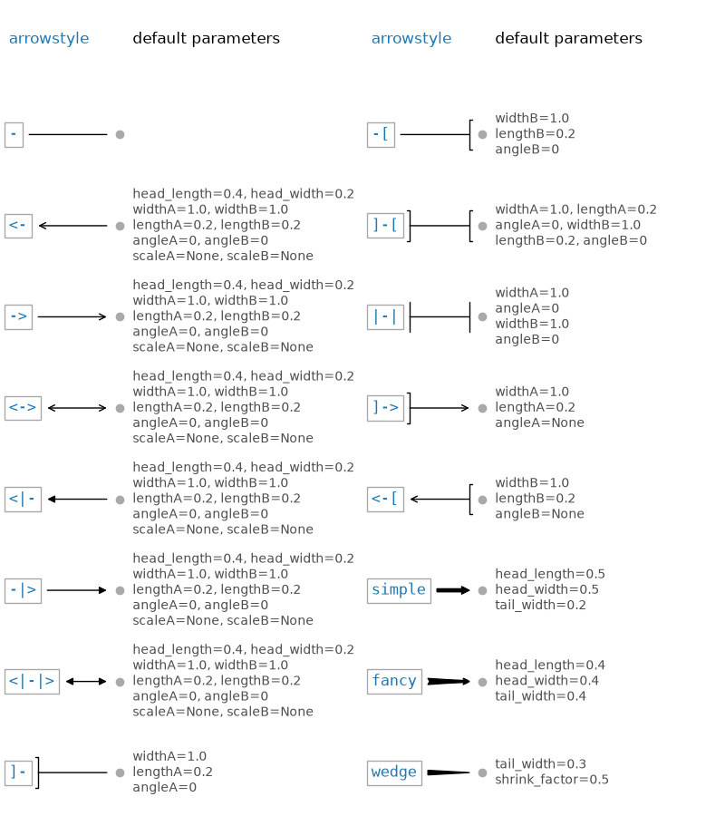
text_labels_and_annotations/fancytextbox_demo
==================
Source
"""
==================
Styling text boxes
==================
This example shows how to style text boxes using *bbox* parameters.
"""
import matplotlib.pyplot as plt
plt.text(0.6, 0.7, "eggs", size=50, rotation=30.,
ha="center", va="center",
bbox=dict(boxstyle="round",
ec=(1., 0.5, 0.5),
fc=(1., 0.8, 0.8),
)
)
plt.text(0.55, 0.6, "spam", size=50, rotation=-25.,
ha="right", va="top",
bbox=dict(boxstyle="square",
ec=(1., 0.5, 0.5),
fc=(1., 0.8, 0.8),
)
)
plt.show()
text_labels_and_annotations/figlegend_demo
==================
Source
""" ================== Figure legend demo ================== Rather than plotting a legend on each axis, a legend for all the artists on all the sub-axes of a figure can be plotted instead. """ import matplotlib.pyplot as plt import numpy as np fig, axs = plt.subplots(1, 2, layout='constrained') x = np.arange(0.0, 4*np.pi, 0.2) axs[0].plot(x, np.sin(x), label='Line 1') axs[0].plot(x, np.exp(-x/2), marker='o', label='Line 2') axs[1].plot(x, np.sin(x), color='tab:green', label='Line 3') axs[1].plot(x, np.exp(-x/4), color='tab:red', marker='^', label='Line 4') fig.legend(loc='outside right upper') plt.show() # %% # The outside positioning is discussed in detail here: # https://matplotlib.org/stable/users/explain/axes/legend_guide.html#figure-legends # # # .. seealso:: # # The :ref:`legend_guide` contains an in depth discussion on the configuration # options for legends.
text_labels_and_annotations/font_family_rc
=========================
Source
"""
=========================
Configure the font family
=========================
You can explicitly set which font family is picked up, either by specifying
family names of fonts installed on user's system, or generic-families
(e.g., 'serif', 'sans-serif', 'monospace', 'fantasy' or 'cursive'),
or a combination of both.
(see :ref:`text_props`)
In the example below, we are overriding the default sans-serif generic family
to include a specific (Tahoma) font. (Note that the best way to achieve this
would simply be to prepend 'Tahoma' in 'font.family')
The default family is set with the font.family rcparam,
e.g. ::
rcParams['font.family'] = 'sans-serif'
and for the font.family you set a list of font styles to try to find
in order::
rcParams['font.sans-serif'] = ['Tahoma', 'DejaVu Sans',
'Lucida Grande', 'Verdana']
.. redirect-from:: /gallery/font_family_rc_sgskip
The ``font.family`` defaults are OS dependent and can be viewed with:
"""
import matplotlib.pyplot as plt
print(plt.rcParams["font.sans-serif"][0])
print(plt.rcParams["font.monospace"][0])
# %%
# Choose default sans-serif font
def print_text(text):
fig, ax = plt.subplots(figsize=(6, 1), facecolor="#eefade")
ax.text(0.5, 0.5, text, ha='center', va='center', size=40)
ax.axis("off")
plt.show()
plt.rcParams["font.family"] = "sans-serif"
print_text("Hello World! 01")
# %%
# Choose sans-serif font and specify to it to "Nimbus Sans"
plt.rcParams["font.family"] = "sans-serif"
plt.rcParams["font.sans-serif"] = ["Nimbus Sans"]
print_text("Hello World! 02")
# %%
# Choose default monospace font
plt.rcParams["font.family"] = "monospace"
print_text("Hello World! 03")
# %%
# Choose monospace font and specify to it to "FreeMono"
plt.rcParams["font.family"] = "monospace"
plt.rcParams["font.monospace"] = ["FreeMono"]
print_text("Hello World! 04")


text_labels_and_annotations/font_file
====================
Source
r"""
====================
Using ttf font files
====================
Although it is usually not a good idea to explicitly point to a single ttf file
for a font instance, you can do so by passing a `pathlib.Path` instance as the
*font* parameter. Note that passing paths as `str`\s is intentionally not
supported, but you can simply wrap `str`\s in `pathlib.Path`\s as needed.
Here, we use the Computer Modern roman font (``cmr10``) shipped with
Matplotlib.
For a more flexible solution, see
:doc:`/gallery/text_labels_and_annotations/font_family_rc` and
:doc:`/gallery/text_labels_and_annotations/fonts_demo`.
"""
from pathlib import Path
import matplotlib.pyplot as plt
import matplotlib as mpl
fig, ax = plt.subplots()
fpath = Path(mpl.get_data_path(), "fonts/ttf/cmr10.ttf")
ax.set_title(f'This is a special font: {fpath.name}', font=fpath)
ax.set_xlabel('This is the default font')
plt.show()
# %%
#
# .. admonition:: References
#
# The use of the following functions, methods, classes and modules is shown
# in this example:
#
# - `matplotlib.axes.Axes.set_title`
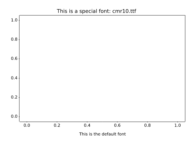
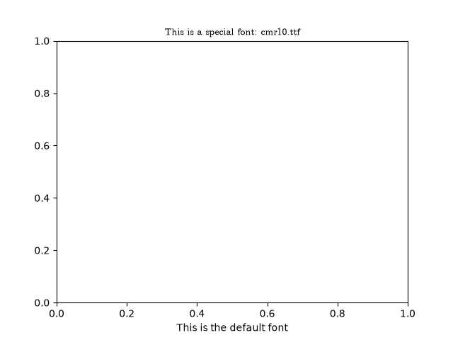
text_labels_and_annotations/font_table
==========
Source
"""
==========
Font table
==========
Matplotlib's font support is provided by the FreeType library.
Here, we use `~.Axes.table` to draw a table that shows the glyphs by Unicode
codepoint. For brevity, the table only contains the first 256 glyphs.
The example is a full working script. You can download it and use it to
investigate a font by running ::
python font_table.py /path/to/font/file
"""
import os
from pathlib import Path
import unicodedata
import matplotlib.pyplot as plt
import matplotlib.font_manager as fm
from matplotlib.ft2font import FT2Font
def print_glyphs(path):
"""
Print the all glyphs in the given font file to stdout.
Parameters
----------
path : str or None
The path to the font file. If None, use Matplotlib's default font.
"""
if path is None:
path = fm.findfont(fm.FontProperties()) # The default font.
font = FT2Font(path)
charmap = font.get_charmap()
max_indices_len = len(str(max(charmap.values())))
print("The font face contains the following glyphs:")
for char_code, glyph_index in charmap.items():
char = chr(char_code)
name = unicodedata.name(
char,
f"{char_code:#x} ({font.get_glyph_name(glyph_index)})")
print(f"{glyph_index:>{max_indices_len}} {char} {name}")
def draw_font_table(path):
"""
Draw a font table of the first 255 chars of the given font.
Parameters
----------
path : str or None
The path to the font file. If None, use Matplotlib's default font.
"""
if path is None:
path = fm.findfont(fm.FontProperties()) # The default font.
font = FT2Font(path)
# A charmap is a mapping of "character codes" (in the sense of a character
# encoding, e.g. latin-1) to glyph indices (i.e. the internal storage table
# of the font face).
# In FreeType>=2.1, a Unicode charmap (i.e. mapping Unicode codepoints)
# is selected by default. Moreover, recent versions of FreeType will
# automatically synthesize such a charmap if the font does not include one
# (this behavior depends on the font format; for example it is present
# since FreeType 2.0 for Type 1 fonts but only since FreeType 2.8 for
# TrueType (actually, SFNT) fonts).
# The code below (specifically, the ``chr(char_code)`` call) assumes that
# we have indeed selected a Unicode charmap.
codes = font.get_charmap().items()
labelc = [f"{i:X}" for i in range(16)]
labelr = [f"{i:02X}" for i in range(0, 16*16, 16)]
chars = [["" for c in range(16)] for r in range(16)]
for char_code, glyph_index in codes:
if char_code >= 256:
continue
row, col = divmod(char_code, 16)
chars[row][col] = chr(char_code)
fig, ax = plt.subplots(figsize=(8, 4))
ax.set_title(os.path.basename(path))
ax.set_axis_off()
table = ax.table(
cellText=chars,
rowLabels=labelr,
colLabels=labelc,
rowColours=["palegreen"] * 16,
colColours=["palegreen"] * 16,
cellColours=[[".95" for c in range(16)] for r in range(16)],
cellLoc='center',
loc='upper left',
)
for key, cell in table.get_celld().items():
row, col = key
if row > 0 and col > -1: # Beware of table's idiosyncratic indexing...
cell.set_text_props(font=Path(path))
fig.tight_layout()
plt.show()
if __name__ == "__main__":
from argparse import ArgumentParser
parser = ArgumentParser(description="Display a font table.")
parser.add_argument("path", nargs="?", help="Path to the font file.")
parser.add_argument("--print-all", action="store_true",
help="Additionally, print all chars to stdout.")
args = parser.parse_args()
if args.print_all:
print_glyphs(args.path)
draw_font_table(args.path)
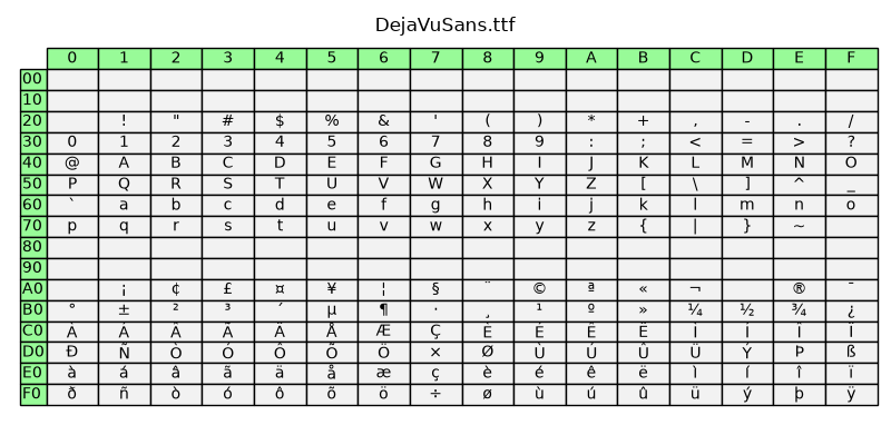
text_labels_and_annotations/fonts_demo
==================================
Source
"""
==================================
Fonts demo (object-oriented style)
==================================
Set font properties using setters.
See :doc:`fonts_demo_kw` to achieve the same effect using keyword arguments.
"""
import matplotlib.pyplot as plt
from matplotlib.font_manager import FontProperties
fig = plt.figure()
alignment = {'horizontalalignment': 'center', 'verticalalignment': 'baseline'}
yp = [0.8, 0.7, 0.6, 0.5, 0.4, 0.3, 0.2]
heading_font = FontProperties(size='large')
# Show family options
fig.text(0.1, 0.9, 'family', fontproperties=heading_font, **alignment)
families = ['serif', 'sans-serif', 'cursive', 'fantasy', 'monospace']
for k, family in enumerate(families):
font = FontProperties(family=[family])
fig.text(0.1, yp[k], family, fontproperties=font, **alignment)
# Show style options
styles = ['normal', 'italic', 'oblique']
fig.text(0.3, 0.9, 'style', fontproperties=heading_font, **alignment)
for k, style in enumerate(styles):
font = FontProperties(family='sans-serif', style=style)
fig.text(0.3, yp[k], style, fontproperties=font, **alignment)
# Show variant options
variants = ['normal', 'small-caps']
fig.text(0.5, 0.9, 'variant', fontproperties=heading_font, **alignment)
for k, variant in enumerate(variants):
font = FontProperties(family='serif', variant=variant)
fig.text(0.5, yp[k], variant, fontproperties=font, **alignment)
# Show weight options
weights = ['light', 'normal', 'medium', 'semibold', 'bold', 'heavy', 'black']
fig.text(0.7, 0.9, 'weight', fontproperties=heading_font, **alignment)
for k, weight in enumerate(weights):
font = FontProperties(weight=weight)
fig.text(0.7, yp[k], weight, fontproperties=font, **alignment)
# Show size options
sizes = [
'xx-small', 'x-small', 'small', 'medium', 'large', 'x-large', 'xx-large']
fig.text(0.9, 0.9, 'size', fontproperties=heading_font, **alignment)
for k, size in enumerate(sizes):
font = FontProperties(size=size)
fig.text(0.9, yp[k], size, fontproperties=font, **alignment)
# Show bold italic
font = FontProperties(style='italic', weight='bold', size='x-small')
fig.text(0.3, 0.1, 'bold italic', fontproperties=font, **alignment)
font = FontProperties(style='italic', weight='bold', size='medium')
fig.text(0.3, 0.2, 'bold italic', fontproperties=font, **alignment)
font = FontProperties(style='italic', weight='bold', size='x-large')
fig.text(0.3, 0.3, 'bold italic', fontproperties=font, **alignment)
plt.show()
text_labels_and_annotations/fonts_demo_kw
==============================
Source
"""
==============================
Fonts demo (keyword arguments)
==============================
Set font properties using keyword arguments.
See :doc:`fonts_demo` to achieve the same effect using setters.
"""
import matplotlib.pyplot as plt
fig = plt.figure()
alignment = {'horizontalalignment': 'center', 'verticalalignment': 'baseline'}
yp = [0.8, 0.7, 0.6, 0.5, 0.4, 0.3, 0.2]
# Show family options
fig.text(0.1, 0.9, 'family', size='large', **alignment)
families = ['serif', 'sans-serif', 'cursive', 'fantasy', 'monospace']
for k, family in enumerate(families):
fig.text(0.1, yp[k], family, family=family, **alignment)
# Show style options
fig.text(0.3, 0.9, 'style', **alignment)
styles = ['normal', 'italic', 'oblique']
for k, style in enumerate(styles):
fig.text(0.3, yp[k], style, family='sans-serif', style=style, **alignment)
# Show variant options
fig.text(0.5, 0.9, 'variant', **alignment)
variants = ['normal', 'small-caps']
for k, variant in enumerate(variants):
fig.text(0.5, yp[k], variant, family='serif', variant=variant, **alignment)
# Show weight options
fig.text(0.7, 0.9, 'weight', **alignment)
weights = ['light', 'normal', 'medium', 'semibold', 'bold', 'heavy', 'black']
for k, weight in enumerate(weights):
fig.text(0.7, yp[k], weight, weight=weight, **alignment)
# Show size options
fig.text(0.9, 0.9, 'size', **alignment)
sizes = [
'xx-small', 'x-small', 'small', 'medium', 'large', 'x-large', 'xx-large']
for k, size in enumerate(sizes):
fig.text(0.9, yp[k], size, size=size, **alignment)
# Show bold italic
fig.text(0.3, 0.1, 'bold italic',
style='italic', weight='bold', size='x-small', **alignment)
fig.text(0.3, 0.2, 'bold italic',
style='italic', weight='bold', size='medium', **alignment)
fig.text(0.3, 0.3, 'bold italic',
style='italic', weight='bold', size='x-large', **alignment)
plt.show()
text_labels_and_annotations/label_subplots
==================
Source
"""
==================
Labelling subplots
==================
Labelling subplots is relatively straightforward, and varies, so Matplotlib
does not have a general method for doing this.
We showcase two methods to position text at a given physical offset (in
fontsize units or in points) away from a corner of the Axes: one using
`~.Axes.annotate`, and one using `.ScaledTranslation`.
For convenience, this example uses `.pyplot.subplot_mosaic` and subplot
labels as keys for the subplots. However, the approach also works with
`.pyplot.subplots` or keys that are different from what you want to label the
subplot with.
"""
import matplotlib.pyplot as plt
from matplotlib.transforms import ScaledTranslation
# %%
fig, axs = plt.subplot_mosaic([['a)', 'c)'], ['b)', 'c)'], ['d)', 'd)']],
layout='constrained')
for label, ax in axs.items():
# Use Axes.annotate to put the label
# - at the top left corner (axes fraction (0, 1)),
# - offset half-a-fontsize right and half-a-fontsize down
# (offset fontsize (+0.5, -0.5)),
# i.e. just inside the axes.
ax.annotate(
label,
xy=(0, 1), xycoords='axes fraction',
xytext=(+0.5, -0.5), textcoords='offset fontsize',
fontsize='medium', verticalalignment='top', fontfamily='serif',
bbox=dict(facecolor='0.7', edgecolor='none', pad=3.0))
# %%
fig, axs = plt.subplot_mosaic([['a)', 'c)'], ['b)', 'c)'], ['d)', 'd)']],
layout='constrained')
for label, ax in axs.items():
# Use ScaledTranslation to put the label
# - at the top left corner (axes fraction (0, 1)),
# - offset 20 pixels left and 7 pixels up (offset points (-20, +7)),
# i.e. just outside the axes.
ax.text(
0.0, 1.0, label, transform=(
ax.transAxes + ScaledTranslation(-20/72, +7/72, fig.dpi_scale_trans)),
fontsize='medium', va='bottom', fontfamily='serif')
# %%
# If we want it aligned with the title, either incorporate in the title or
# use the *loc* keyword argument:
fig, axs = plt.subplot_mosaic([['a)', 'c)'], ['b)', 'c)'], ['d)', 'd)']],
layout='constrained')
for label, ax in axs.items():
ax.set_title('Normal Title', fontstyle='italic')
ax.set_title(label, fontfamily='serif', loc='left', fontsize='medium')
plt.show()
# %%
#
# .. admonition:: References
#
# The use of the following functions, methods, classes and modules is shown
# in this example:
#
# - `matplotlib.figure.Figure.subplot_mosaic` /
# `matplotlib.pyplot.subplot_mosaic`
# - `matplotlib.axes.Axes.set_title`
# - `matplotlib.axes.Axes.annotate`
text_labels_and_annotations/legend
===============================
Source
"""
===============================
Legend using pre-defined labels
===============================
Defining legend labels with plots.
"""
import matplotlib.pyplot as plt
import numpy as np
# Make some fake data.
a = b = np.arange(0, 3, .02)
c = np.exp(a)
d = c[::-1]
# Create plots with pre-defined labels.
fig, ax = plt.subplots()
ax.plot(a, c, 'k--', label='Model length')
ax.plot(a, d, 'k:', label='Data length')
ax.plot(a, c + d, 'k', label='Total message length')
legend = ax.legend(loc='upper center', shadow=True, fontsize='x-large')
# Put a nicer background color on the legend.
legend.get_frame().set_facecolor('C0')
plt.show()
# %%
#
# .. admonition:: References
#
# The use of the following functions, methods, classes and modules is shown
# in this example:
#
# - `matplotlib.axes.Axes.plot` / `matplotlib.pyplot.plot`
# - `matplotlib.axes.Axes.legend` / `matplotlib.pyplot.legend`
#
# .. seealso::
#
# The :ref:`legend_guide` contains an in depth discussion on the configuration
# options for legends.
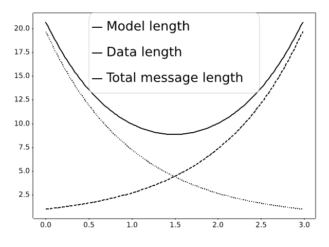
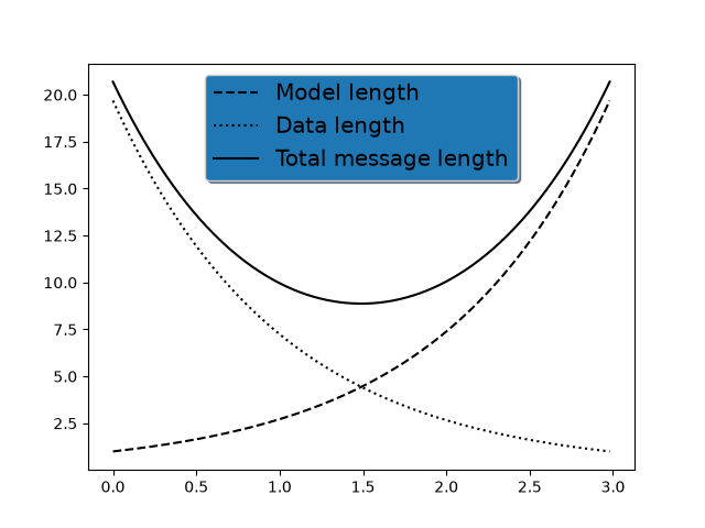
text_labels_and_annotations/legend_demo
===========
Source
"""
===========
Legend Demo
===========
There are many ways to create and customize legends in Matplotlib. Below
we'll show a few examples for how to do so.
First we'll show off how to make a legend for specific lines.
"""
import matplotlib.pyplot as plt
import numpy as np
import matplotlib.collections as mcol
from matplotlib.legend_handler import HandlerLineCollection, HandlerTuple
from matplotlib.lines import Line2D
t1 = np.arange(0.0, 2.0, 0.1)
t2 = np.arange(0.0, 2.0, 0.01)
fig, ax = plt.subplots()
# note that plot returns a list of lines. The "l1, = plot" usage
# extracts the first element of the list into l1 using tuple
# unpacking. So l1 is a Line2D instance, not a sequence of lines
l1, = ax.plot(t2, np.exp(-t2))
l2, l3 = ax.plot(t2, np.sin(2 * np.pi * t2), '--o', t1, np.log(1 + t1), '.')
l4, = ax.plot(t2, np.exp(-t2) * np.sin(2 * np.pi * t2), 's-.')
ax.legend((l2, l4), ('oscillatory', 'damped'), loc='upper right', shadow=True)
ax.set_xlabel('time')
ax.set_ylabel('volts')
ax.set_title('Damped oscillation')
plt.show()
# %%
# Next we'll demonstrate plotting more complex labels.
x = np.linspace(0, 1)
fig, (ax0, ax1) = plt.subplots(2, 1)
# Plot the lines y=x**n for n=1..4.
for n in range(1, 5):
ax0.plot(x, x**n, label=f"{n=}")
leg = ax0.legend(loc="upper left", bbox_to_anchor=[0, 1],
ncols=2, shadow=True, title="Legend", fancybox=True)
leg.get_title().set_color("red")
# Demonstrate some more complex labels.
ax1.plot(x, x**2, label="multi\nline")
half_pi = np.linspace(0, np.pi / 2)
ax1.plot(np.sin(half_pi), np.cos(half_pi), label=r"$\frac{1}{2}\pi$")
ax1.plot(x, 2**(x**2), label="$2^{x^2}$")
ax1.legend(shadow=True, fancybox=True)
plt.show()
# %%
# Here we attach legends to more complex plots.
fig, axs = plt.subplots(3, 1, layout="constrained")
top_ax, middle_ax, bottom_ax = axs
top_ax.bar([0, 1, 2], [0.2, 0.3, 0.1], width=0.4, label="Bar 1",
align="center")
top_ax.bar([0.5, 1.5, 2.5], [0.3, 0.2, 0.2], color="red", width=0.4,
label="Bar 2", align="center")
top_ax.legend()
middle_ax.errorbar([0, 1, 2], [2, 3, 1], xerr=0.4, fmt="s", label="test 1")
middle_ax.errorbar([0, 1, 2], [3, 2, 4], yerr=0.3, fmt="o", label="test 2")
middle_ax.errorbar([0, 1, 2], [1, 1, 3], xerr=0.4, yerr=0.3, fmt="^",
label="test 3")
middle_ax.legend()
bottom_ax.stem([0.3, 1.5, 2.7], [1, 3.6, 2.7], label="stem test")
bottom_ax.legend()
plt.show()
# %%
# Now we'll showcase legend entries with more than one legend key.
fig, (ax1, ax2) = plt.subplots(2, 1, layout='constrained')
# First plot: two legend keys for a single entry
p1 = ax1.scatter([1], [5], c='r', marker='s', s=100)
p2 = ax1.scatter([3], [2], c='b', marker='o', s=100)
# `plot` returns a list, but we want the handle - thus the comma on the left
p3, = ax1.plot([1, 5], [4, 4], 'm-d')
# Assign two of the handles to the same legend entry by putting them in a tuple
# and using a generic handler map (which would be used for any additional
# tuples of handles like (p1, p3)).
l = ax1.legend([(p1, p3), p2], ['two keys', 'one key'], scatterpoints=1,
numpoints=1, handler_map={tuple: HandlerTuple(ndivide=None)})
# Second plot: plot two bar charts on top of each other and change the padding
# between the legend keys
x_left = [1, 2, 3]
y_pos = [1, 3, 2]
y_neg = [2, 1, 4]
rneg = ax2.bar(x_left, y_neg, width=0.5, color='w', hatch='///', label='-1')
rpos = ax2.bar(x_left, y_pos, width=0.5, color='k', label='+1')
# Treat each legend entry differently by using specific `HandlerTuple`s
l = ax2.legend([(rpos, rneg), (rneg, rpos)], ['pad!=0', 'pad=0'],
handler_map={(rpos, rneg): HandlerTuple(ndivide=None),
(rneg, rpos): HandlerTuple(ndivide=None, pad=0.)})
plt.show()
# %%
# Finally, it is also possible to write custom classes that define
# how to stylize legends.
class HandlerDashedLines(HandlerLineCollection):
"""
Custom Handler for LineCollection instances.
"""
def create_artists(self, legend, orig_handle,
xdescent, ydescent, width, height, fontsize, trans):
# figure out how many lines there are
numlines = len(orig_handle.get_segments())
xdata, xdata_marker = self.get_xdata(legend, xdescent, ydescent,
width, height, fontsize)
leglines = []
# divide the vertical space where the lines will go
# into equal parts based on the number of lines
ydata = np.full_like(xdata, height / (numlines + 1))
# for each line, create the line at the proper location
# and set the dash pattern
for i in range(numlines):
legline = Line2D(xdata, ydata * (numlines - i) - ydescent)
self.update_prop(legline, orig_handle, legend)
# set color, dash pattern, and linewidth to that
# of the lines in linecollection
try:
color = orig_handle.get_colors()[i]
except IndexError:
color = orig_handle.get_colors()[0]
try:
dashes = orig_handle.get_dashes()[i]
except IndexError:
dashes = orig_handle.get_dashes()[0]
try:
lw = orig_handle.get_linewidths()[i]
except IndexError:
lw = orig_handle.get_linewidths()[0]
if dashes[1] is not None:
legline.set_dashes(dashes[1])
legline.set_color(color)
legline.set_transform(trans)
legline.set_linewidth(lw)
leglines.append(legline)
return leglines
x = np.linspace(0, 5, 100)
fig, ax = plt.subplots()
colors = plt.rcParams['axes.prop_cycle'].by_key()['color'][:5]
styles = ['solid', 'dashed', 'dashed', 'dashed', 'solid']
for i, color, style in zip(range(5), colors, styles):
ax.plot(x, np.sin(x) - .1 * i, c=color, ls=style)
# make proxy artists
# make list of one line -- doesn't matter what the coordinates are
line = [[(0, 0)]]
# set up the proxy artist
lc = mcol.LineCollection(5 * line, linestyles=styles, colors=colors)
# create the legend
ax.legend([lc], ['multi-line'], handler_map={type(lc): HandlerDashedLines()},
handlelength=2.5, handleheight=3)
plt.show()
# %%
#
# .. seealso::
#
# The :ref:`legend_guide` contains an in depth discussion on the configuration
# options for legends.
text_labels_and_annotations/line_with_text
=======================
Source
"""
=======================
Artist within an artist
=======================
Override basic methods so an artist can contain another
artist. In this case, the line contains a Text instance to label it.
"""
import matplotlib.pyplot as plt
import numpy as np
import matplotlib.lines as lines
import matplotlib.text as mtext
import matplotlib.transforms as mtransforms
class MyLine(lines.Line2D):
def __init__(self, *args, **kwargs):
# we'll update the position when the line data is set
self.text = mtext.Text(0, 0, '')
super().__init__(*args, **kwargs)
# we can't access the label attr until *after* the line is
# initiated
self.text.set_text(self.get_label())
def set_figure(self, figure):
self.text.set_figure(figure)
super().set_figure(figure)
# Override the Axes property setter to set Axes on our children as well.
@lines.Line2D.axes.setter
def axes(self, new_axes):
self.text.axes = new_axes
lines.Line2D.axes.fset(self, new_axes) # Call the superclass property setter.
def set_transform(self, transform):
# 2 pixel offset
texttrans = transform + mtransforms.Affine2D().translate(2, 2)
self.text.set_transform(texttrans)
super().set_transform(transform)
def set_data(self, x, y):
if len(x):
self.text.set_position((x[-1], y[-1]))
super().set_data(x, y)
def draw(self, renderer):
# draw my label at the end of the line with 2 pixel offset
super().draw(renderer)
self.text.draw(renderer)
# Fixing random state for reproducibility
np.random.seed(19680801)
fig, ax = plt.subplots()
x, y = np.random.rand(2, 20)
line = MyLine(x, y, mfc='red', ms=12, label='line label')
line.text.set_color('red')
line.text.set_fontsize(16)
ax.add_line(line)
plt.show()
# %%
#
# .. admonition:: References
#
# The use of the following functions, methods, classes and modules is shown
# in this example:
#
# - `matplotlib.lines`
# - `matplotlib.lines.Line2D`
# - `matplotlib.lines.Line2D.set_data`
# - `matplotlib.artist`
# - `matplotlib.artist.Artist`
# - `matplotlib.artist.Artist.draw`
# - `matplotlib.artist.Artist.set_transform`
# - `matplotlib.text`
# - `matplotlib.text.Text`
# - `matplotlib.text.Text.set_color`
# - `matplotlib.text.Text.set_fontsize`
# - `matplotlib.text.Text.set_position`
# - `matplotlib.axes.Axes.add_line`
# - `matplotlib.transforms`
# - `matplotlib.transforms.Affine2D`
text_labels_and_annotations/mathtext_asarray
=======================
Source
"""
=======================
Convert texts to images
=======================
"""
from io import BytesIO
from PIL import Image
import matplotlib.pyplot as plt
import numpy as np
from matplotlib.figure import Figure
from matplotlib.transforms import IdentityTransform
def text_to_rgba(s, *, dpi, **kwargs):
# To convert a text string to an image, we can:
# - draw it on an empty and transparent figure;
# - save the figure to a temporary buffer using ``bbox_inches="tight",
# pad_inches=0`` which will pick the correct area to save;
# - load the buffer using ``PIL.Image.open``.
#
# (If desired, one can also directly save the image to the filesystem.)
fig = Figure(facecolor="none")
fig.text(0, 0, s, **kwargs)
with BytesIO() as buf:
fig.savefig(buf, dpi=dpi, format="png", bbox_inches="tight",
pad_inches=0)
buf.seek(0)
rgba = np.asarray(Image.open(buf))
return rgba
fig = plt.figure()
rgba1 = text_to_rgba(r"IQ: $\sigma_i=15$", color="blue", fontsize=20, dpi=200)
rgba2 = text_to_rgba(r"some other string", color="red", fontsize=20, dpi=200)
# One can then draw such text images to a Figure using `.Figure.figimage`.
fig.figimage(rgba1, 100, 50)
fig.figimage(rgba2, 100, 150)
# One can also directly draw texts to a figure with positioning
# in pixel coordinates by using `.Figure.text` together with
# `.transforms.IdentityTransform`.
fig.text(100, 250, r"IQ: $\sigma_i=15$", color="blue", fontsize=20,
transform=IdentityTransform())
fig.text(100, 350, r"some other string", color="red", fontsize=20,
transform=IdentityTransform())
plt.show()
# %%
#
# .. admonition:: References
#
# The use of the following functions, methods, classes and modules is shown
# in this example:
#
# - `matplotlib.figure.Figure.figimage`
# - `matplotlib.figure.Figure.text`
# - `matplotlib.transforms.IdentityTransform`
# - `matplotlib.image.imread`
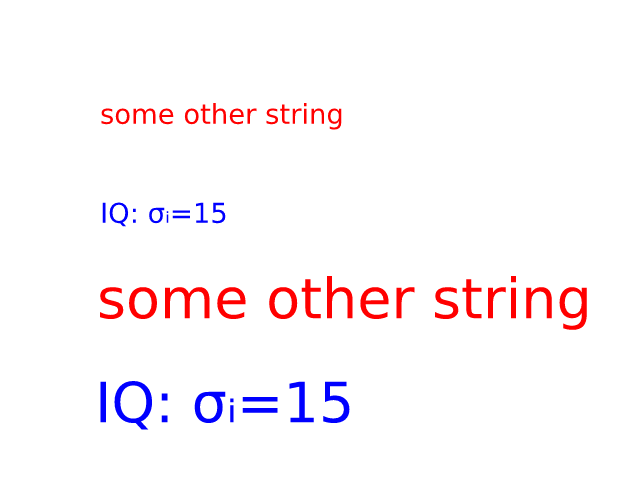
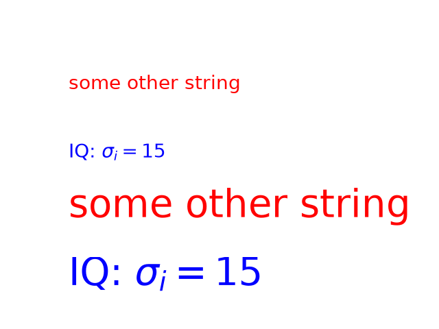
text_labels_and_annotations/mathtext_demo
========
Source
"""
========
Mathtext
========
Use Matplotlib's internal LaTeX parser and layout engine. For true LaTeX
rendering, see the text.usetex option.
"""
import matplotlib.pyplot as plt
fig, ax = plt.subplots()
ax.plot([1, 2, 3], label=r'$\sqrt{x^2}$')
ax.legend()
ax.set_xlabel(r'$\Delta_i^j$', fontsize=20)
ax.set_ylabel(r'$\Delta_{i+1}^j$', fontsize=20)
ax.set_title(r'$\Delta_i^j \hspace{0.4} \mathrm{versus} \hspace{0.4} '
r'\Delta_{i+1}^j$', fontsize=20)
tex = r'$\mathcal{R}\prod_{i=\alpha_{i+1}}^\infty a_i\sin(2 \pi f x_i)$'
ax.text(1, 1.6, tex, fontsize=20, va='bottom')
fig.tight_layout()
plt.show()
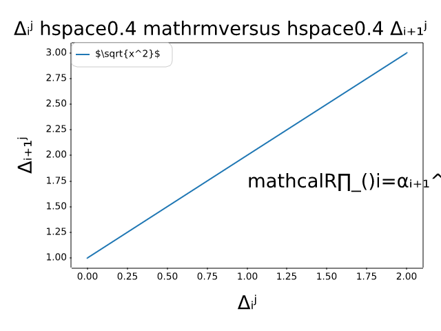
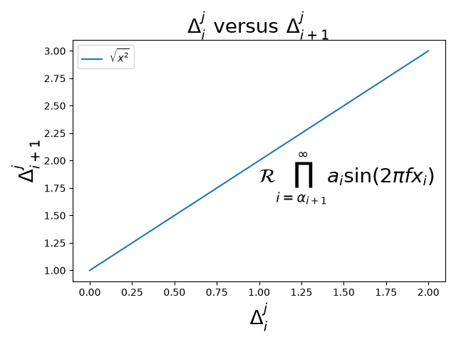
text_labels_and_annotations/mathtext_examples
========================
Source
"""
========================
Mathematical expressions
========================
Selected features of Matplotlib's math rendering engine.
"""
import re
import subprocess
import sys
import matplotlib.pyplot as plt
# Selection of features following "Writing mathematical expressions" tutorial,
# with randomly picked examples.
mathtext_demos = {
"Header demo":
r"$W^{3\beta}_{\delta_1 \rho_1 \sigma_2} = "
r"U^{3\beta}_{\delta_1 \rho_1} + \frac{1}{8 \pi 2} "
r"\int^{\alpha_2}_{\alpha_2} d \alpha^\prime_2 \left[\frac{ "
r"U^{2\beta}_{\delta_1 \rho_1} - \alpha^\prime_2U^{1\beta}_"
r"{\rho_1 \sigma_2} }{U^{0\beta}_{\rho_1 \sigma_2}}\right]$",
"Subscripts and superscripts":
r"$\alpha_i > \beta_i,\ "
r"\alpha_{i+1}^j = {\rm sin}(2\pi f_j t_i) e^{-5 t_i/\tau},\ "
r"\ldots$",
"Fractions, binomials and stacked numbers":
r"$\frac{3}{4},\ \binom{3}{4},\ \genfrac{}{}{0}{}{3}{4},\ "
r"\left(\frac{5 - \frac{1}{x}}{4}\right),\ \ldots$",
"Radicals":
r"$\sqrt{2},\ \sqrt[3]{x},\ \ldots$",
"Fonts":
r"$\mathrm{Roman}\ , \ \mathit{Italic}\ , \ \mathtt{Typewriter} \ "
r"\mathrm{or}\ \mathcal{CALLIGRAPHY}$",
"Accents":
r"$\acute a,\ \bar a,\ \breve a,\ \dot a,\ \ddot a, \ \grave a, \ "
r"\hat a,\ \tilde a,\ \vec a,\ \widehat{xyz},\ \widetilde{xyz},\ "
r"\ldots$",
"Greek, Hebrew":
r"$\alpha,\ \beta,\ \chi,\ \delta,\ \lambda,\ \mu,\ "
r"\Delta,\ \Gamma,\ \Omega,\ \Phi,\ \Pi,\ \Upsilon,\ \nabla,\ "
r"\aleph,\ \beth,\ \daleth,\ \gimel,\ \ldots$",
"Delimiters, functions and Symbols":
r"$\coprod,\ \int,\ \oint,\ \prod,\ \sum,\ "
r"\log,\ \sin,\ \approx,\ \oplus,\ \star,\ \varpropto,\ "
r"\infty,\ \partial,\ \Re,\ \leftrightsquigarrow, \ \ldots$",
}
n_lines = len(mathtext_demos)
def doall():
# Colors used in Matplotlib online documentation.
mpl_grey_rgb = (51 / 255, 51 / 255, 51 / 255)
# Creating figure and axis.
fig = plt.figure(figsize=(7, 7))
ax = fig.add_axes((0.01, 0.01, 0.98, 0.90),
facecolor="white", frameon=True)
ax.set_xlim(0, 1)
ax.set_ylim(0, 1)
ax.set_title("Matplotlib's math rendering engine",
color=mpl_grey_rgb, fontsize=14, weight='bold')
ax.set_xticks([])
ax.set_yticks([])
# Gap between lines in axes coords
line_axesfrac = 1 / n_lines
# Plot header demonstration formula.
full_demo = mathtext_demos['Header demo']
ax.annotate(full_demo,
xy=(0.5, 1. - 0.59 * line_axesfrac),
color='tab:orange', ha='center', fontsize=20)
# Plot feature demonstration formulae.
for i_line, (title, demo) in enumerate(mathtext_demos.items()):
print(i_line, demo)
if i_line == 0:
continue
baseline = 1 - i_line * line_axesfrac
baseline_next = baseline - line_axesfrac
fill_color = ['white', 'tab:blue'][i_line % 2]
ax.axhspan(baseline, baseline_next, color=fill_color, alpha=0.2)
ax.annotate(f'{title}:',
xy=(0.06, baseline - 0.3 * line_axesfrac),
color=mpl_grey_rgb, weight='bold')
ax.annotate(demo,
xy=(0.04, baseline - 0.75 * line_axesfrac),
color=mpl_grey_rgb, fontsize=16)
plt.show()
if '--latex' in sys.argv:
# Run: python mathtext_examples.py --latex
# Need amsmath and amssymb packages.
with open("mathtext_examples.ltx", "w") as fd:
fd.write("\\documentclass{article}\n")
fd.write("\\usepackage{amsmath, amssymb}\n")
fd.write("\\begin{document}\n")
fd.write("\\begin{enumerate}\n")
for s in mathtext_demos.values():
s = re.sub(r"(?<!\\)\$", "$$", s)
fd.write("\\item %s\n" % s)
fd.write("\\end{enumerate}\n")
fd.write("\\end{document}\n")
subprocess.call(["pdflatex", "mathtext_examples.ltx"])
else:
doall()
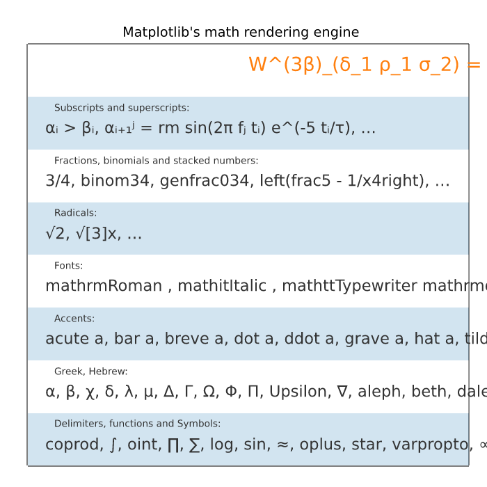
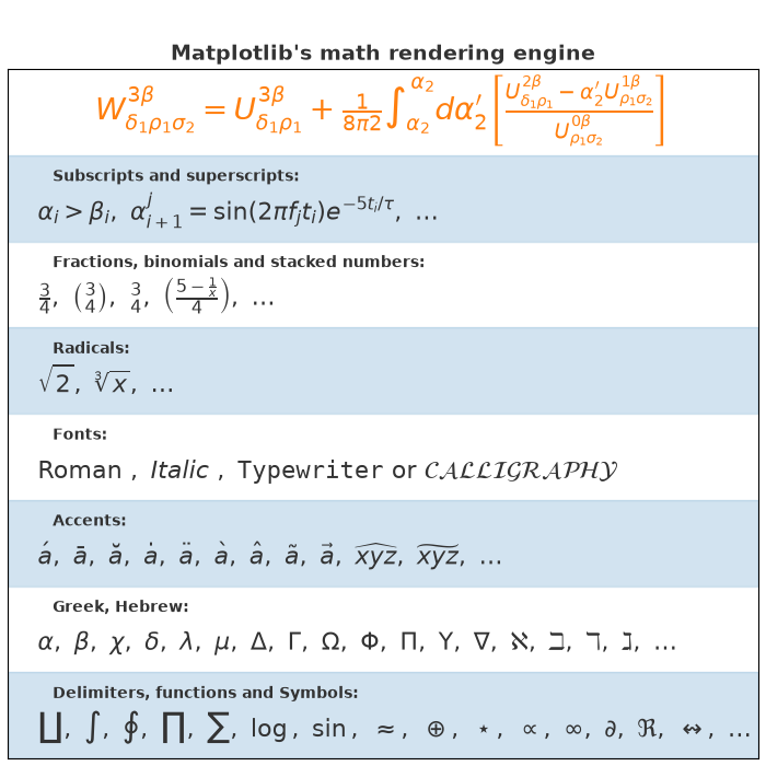
text_labels_and_annotations/mathtext_fontfamily_example
===============
Source
"""
===============
Math fontfamily
===============
A simple example showcasing the new *math_fontfamily* parameter that can
be used to change the family of fonts for each individual text
element in a plot.
If no parameter is set, the global value
:rc:`mathtext.fontset` will be used.
"""
import matplotlib.pyplot as plt
fig, ax = plt.subplots(figsize=(6, 5))
# A simple plot for the background.
ax.plot(range(11), color="0.9")
# A text mixing normal text and math text.
msg = (r"Normal Text. $Text\ in\ math\ mode:\ "
r"\int_{0}^{\infty } x^2 dx$")
# Set the text in the plot.
ax.text(1, 7, msg, size=12, math_fontfamily='cm')
# Set another font for the next text.
ax.text(1, 3, msg, size=12, math_fontfamily='dejavuserif')
# *math_fontfamily* can be used in most places where there is text,
# like in the title:
ax.set_title(r"$Title\ in\ math\ mode:\ \int_{0}^{\infty } x^2 dx$",
math_fontfamily='stixsans', size=14)
# Note that the normal text is not changed by *math_fontfamily*.
plt.show()
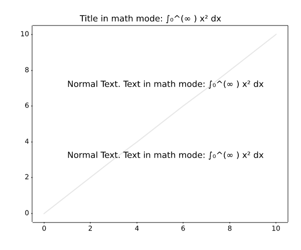
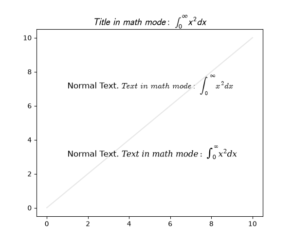
text_labels_and_annotations/multiline
==============
Source
"""
==============
Multiline text
==============
Texts may contain newlines to create multiline text.
The text alignment of the individual lines can be controlled by the
``multialignment`` parameter. If not set, the alignment of the lines is inferred from
the ``horizontalalignment`` and ``verticalalignment`` parameters, which primarily
control the alignment of the bounding box of the text to its anchor point; e.g. if the
text has the anchor point to its right, all text lines will be aligned to the right
so that they pick up that anchor point.
When using mutli-line labels, it is recommended to use a layout manager (e.g.
``layout="constrained"``) to ensure that there is enough space for the labels..
"""
import matplotlib.pyplot as plt
fig, ax = plt.subplots(layout="constrained")
ax.bar(range(6), [0.3, 0.5, 0.8, 1.5, 2.5, 8], alpha=0.3)
ax.set_ylabel('labels are centered,\nso is their multi-line text by default')
ax.set_xlabel('xlabel with\nmultialignment="left"', multialignment="left")
ax.text(
4.5, 6,
'these lines\n'
'are right aligned\n'
'because of horizontalalignment',
horizontalalignment='right',
)
ax.text(
4.5, 4,
'but\n'
'we can override this\n'
'with an explicit multialingment="left"',
horizontalalignment='right',
multialignment='left',
)
plt.show()
# %%
# Each line has the same height irrespective of the used characters unless
# there is math text involved, which may need more vertical space
fig, ax = plt.subplots()
ax.text(0.1, 0.4, "Mat\nTTp\n123", size=18,
va="baseline", bbox=dict(fc="none", ec="tab:orange"))
ax.text(0.3, 0.4, "Mag\nTTT\n123", size=18,
va="baseline", bbox=dict(fc="none", ec="tab:orange"))
ax.text(0.5, 0.4, "Mag\nTTT$^{A^A}$\n123", size=18,
va="baseline", bbox=dict(fc="none", ec="tab:orange"))
ax.axhline(0.4)
ax.set_title("test line spacing for multiline text")
ax.set_xlim(0, 0.7)
ax.yaxis.minorticks_on()
ax.yaxis.set_tick_params(which="minor", grid_color="0.9")
ax.grid(which="both")
plt.show()
text_labels_and_annotations/placing_text_boxes
Placing text boxes
Source
"""
Placing text boxes
==================
When decorating Axes with text boxes, two useful tricks are to place the text
in axes coordinates (see :ref:`transforms_tutorial`),
so the text doesn't move around with changes in x or y limits. You
can also use the ``bbox`` property of text to surround the text with a
`~matplotlib.patches.Patch` instance -- the ``bbox`` keyword argument takes a
dictionary with keys that are Patch properties.
"""
import matplotlib.pyplot as plt
import numpy as np
np.random.seed(19680801)
fig, ax = plt.subplots()
x = 30*np.random.randn(10000)
mu = x.mean()
median = np.median(x)
sigma = x.std()
textstr = '\n'.join((
r'$\mu=%.2f$' % (mu, ),
r'$\mathrm{median}=%.2f$' % (median, ),
r'$\sigma=%.2f$' % (sigma, )))
ax.hist(x, 50)
# these are matplotlib.patch.Patch properties
props = dict(boxstyle='round', facecolor='wheat', alpha=0.5)
# place a text box in upper left in axes coords
ax.text(0.05, 0.95, textstr, transform=ax.transAxes, fontsize=14,
verticalalignment='top', bbox=props)
plt.show()
text_labels_and_annotations/rainbow_text
==================================================
Source
"""
==================================================
Concatenate text objects with different properties
==================================================
The example strings together several Text objects with different properties
(e.g., color or font), positioning each one after the other. The first Text
is created directly using `~.Axes.text`; all subsequent ones are created with
`~.Axes.annotate`, which allows positioning the Text's lower left corner at the
lower right corner (``xy=(1, 0)``) of the previous one (``xycoords=text``).
"""
import matplotlib.pyplot as plt
plt.rcParams["font.size"] = 20
ax = plt.figure().add_subplot(xticks=[], yticks=[])
# The first word, created with text().
text = ax.text(.1, .5, "Matplotlib", color="red")
# Subsequent words, positioned with annotate(), relative to the preceding one.
text = ax.annotate(
" says,", xycoords=text, xy=(1, 0), verticalalignment="bottom",
color="gold", weight="bold") # custom properties
text = ax.annotate(
" hello", xycoords=text, xy=(1, 0), verticalalignment="bottom",
color="green", style="italic") # custom properties
text = ax.annotate(
" world!", xycoords=text, xy=(1, 0), verticalalignment="bottom",
color="blue", family="serif") # custom properties
plt.show()
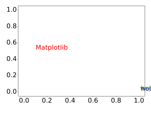
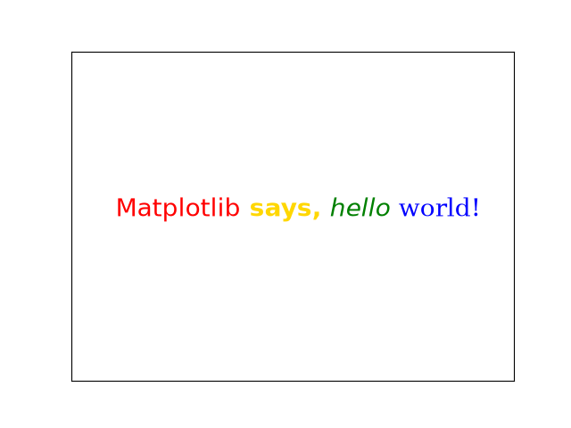
text_labels_and_annotations/stix_fonts_demo
==========
Source
"""
==========
STIX Fonts
==========
Demonstration of `STIX Fonts <https://www.stixfonts.org/>`_ used in LaTeX
rendering.
"""
import matplotlib.pyplot as plt
circle123 = "\N{CIRCLED DIGIT ONE}\N{CIRCLED DIGIT TWO}\N{CIRCLED DIGIT THREE}"
tests = [
r'$%s\;\mathrm{%s}\;\mathbf{%s}$' % ((circle123,) * 3),
r'$\mathsf{Sans \Omega}\;\mathrm{\mathsf{Sans \Omega}}\;'
r'\mathbf{\mathsf{Sans \Omega}}$',
r'$\mathtt{Monospace}$',
r'$\mathcal{CALLIGRAPHIC}$',
r'$\mathbb{Blackboard\;\pi}$',
r'$\mathrm{\mathbb{Blackboard\;\pi}}$',
r'$\mathbf{\mathbb{Blackboard\;\pi}}$',
r'$\mathfrak{Fraktur}\;\mathbf{\mathfrak{Fraktur}}$',
r'$\mathscr{Script}$',
]
fig = plt.figure(figsize=(8, len(tests) + 2))
for i, s in enumerate(tests[::-1]):
fig.text(0, (i + .5) / len(tests), s, fontsize=32)
plt.show()
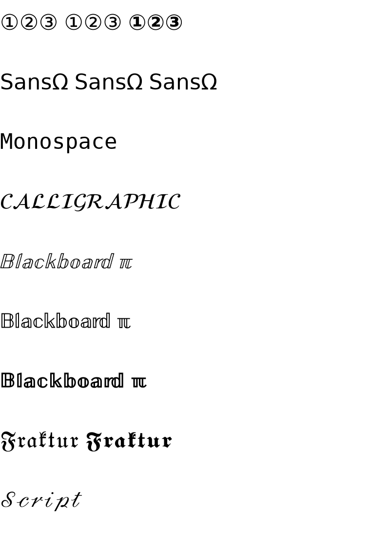
text_labels_and_annotations/tex_demo
===============================
Source
"""
===============================
Render math equations using TeX
===============================
You can use TeX to render all of your Matplotlib text by setting
:rc:`text.usetex` to True. This requires that you have TeX and the other
dependencies described in the :ref:`usetex` tutorial properly
installed on your system. Matplotlib caches processed TeX expressions, so that
only the first occurrence of an expression triggers a TeX compilation. Later
occurrences reuse the rendered image from the cache and are thus faster.
Unicode input is supported, e.g. for the y-axis label in this example.
"""
import matplotlib.pyplot as plt
import numpy as np
plt.rcParams['text.usetex'] = True
t = np.linspace(0.0, 1.0, 100)
s = np.cos(4 * np.pi * t) + 2
fig, ax = plt.subplots(figsize=(6, 4), tight_layout=True)
ax.plot(t, s)
ax.set_xlabel(r'\textbf{time (s)}')
ax.set_ylabel('\\textit{Velocity (\N{DEGREE SIGN}/sec)}', fontsize=16)
ax.set_title(r'\TeX\ is Number $\displaystyle\sum_{n=1}^\infty'
r'\frac{-e^{i\pi}}{2^n}$!', fontsize=16, color='r')
# %%
# A more complex example.
fig, ax = plt.subplots()
# interface tracking profiles
N = 500
delta = 0.6
X = np.linspace(-1, 1, N)
ax.plot(X, (1 - np.tanh(4 * X / delta)) / 2, # phase field tanh profiles
X, (1.4 + np.tanh(4 * X / delta)) / 4, "C2", # composition profile
X, X < 0, "k--") # sharp interface
# legend
ax.legend(("phase field", "level set", "sharp interface"),
shadow=True, loc=(0.01, 0.48), handlelength=1.5, fontsize=16)
# the arrow
ax.annotate("", xy=(-delta / 2., 0.1), xytext=(delta / 2., 0.1),
arrowprops=dict(arrowstyle="<->", connectionstyle="arc3"))
ax.text(0, 0.1, r"$\delta$",
color="black", fontsize=24,
horizontalalignment="center", verticalalignment="center",
bbox=dict(boxstyle="round", fc="white", ec="black", pad=0.2))
# Use tex in labels
ax.set_xticks([-1, 0, 1])
ax.set_xticklabels(["$-1$", r"$\pm 0$", "$+1$"], color="k", size=20)
# Left Y-axis labels, combine math mode and text mode
ax.set_ylabel(r"\bf{phase field} $\phi$", color="C0", fontsize=20)
ax.set_yticks([0, 0.5, 1])
ax.set_yticklabels([r"\bf{0}", r"\bf{.5}", r"\bf{1}"], color="k", size=20)
# Right Y-axis labels
ax.text(1.02, 0.5, r"\bf{level set} $\phi$",
color="C2", fontsize=20, rotation=90,
horizontalalignment="left", verticalalignment="center",
clip_on=False, transform=ax.transAxes)
# Use multiline environment inside a `text`.
# level set equations
eq1 = (r"\begin{eqnarray*}"
r"|\nabla\phi| &=& 1,\\"
r"\frac{\partial \phi}{\partial t} + U|\nabla \phi| &=& 0 "
r"\end{eqnarray*}")
ax.text(1, 0.9, eq1, color="C2", fontsize=18,
horizontalalignment="right", verticalalignment="top")
# phase field equations
eq2 = (r"\begin{eqnarray*}"
r"\mathcal{F} &=& \int f\left( \phi, c \right) dV, \\ "
r"\frac{ \partial \phi } { \partial t } &=& -M_{ \phi } "
r"\frac{ \delta \mathcal{F} } { \delta \phi }"
r"\end{eqnarray*}")
ax.text(0.18, 0.18, eq2, color="C0", fontsize=16)
ax.text(-1, .30, r"gamma: $\gamma$", color="r", fontsize=20)
ax.text(-1, .18, r"Omega: $\Omega$", color="b", fontsize=20)
plt.show()
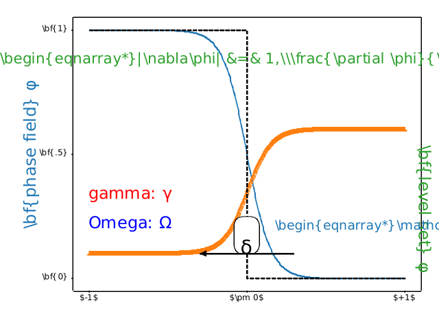
RuntimeError: Failed to process string with tex because latex could not be found
text_labels_and_annotations/text_alignment
==============
Source
"""
==============
Text alignment
==============
Texts are aligned relative to their anchor point depending on the properties
``horizontalalignment`` (default: ``left``) and ``verticalalignment``
(default: ``baseline``.)
.. redirect-from:: /gallery/pyplots/text_layout
.. plot::
import matplotlib.pyplot as plt
import numpy as np
y = [0.22, 0.34, 0.5, 0.56, 0.78]
x = [0.17, 0.5, 0.855]
X, Y = np.meshgrid(x, y)
fig, ax = plt.subplots(figsize=(6, 4), dpi=100)
ax.set(xlim=(0, 1), ylim=(0, 1), xticks=[], yticks=[])
ax.spines[:].set_visible(False)
ax.text(0.5, 0.5, 'plot', fontsize=128, ha='center', va='center', zorder=1)
ax.hlines(y, x[0], x[-1], color='grey')
ax.vlines(x, y[0], y[-1], color='grey')
ax.plot(X.ravel(), Y.ravel(), 'o')
pad_x = 0.02
pad_y = 0.04
ax.text(x[0] - pad_x, y[0], 'bottom', ha='right', va='center')
ax.text(x[0] - pad_x, y[1], 'baseline', ha='right', va='center')
ax.text(x[0] - pad_x, y[2], 'center', ha='right', va='center')
ax.text(x[0] - pad_x, y[3], 'center_baseline', ha='right', va='center')
ax.text(x[0] - pad_x, y[4], 'top', ha='right', va='center')
ax.text(x[0], y[0] - pad_y, 'left', ha='center', va='top')
ax.text(x[1], y[0] - pad_y, 'center', ha='center', va='top')
ax.text(x[2], y[0] - pad_y, 'right', ha='center', va='top')
ax.set_xlabel('horizontalalignment', fontsize=14)
ax.set_ylabel('verticalalignment', fontsize=14, labelpad=35)
ax.set_title(
'Relative position of text anchor point depending on alignment')
plt.show()
"""
# %%
# The following plot uses this to align text relative to a plotted rectangle.
import matplotlib.pyplot as plt
fig, ax = plt.subplots()
# Build a rectangle in axes coords
left, width = .25, .5
bottom, height = .25, .5
right = left + width
top = bottom + height
p = plt.Rectangle((left, bottom), width, height, fill=False)
p.set_transform(ax.transAxes)
p.set_clip_on(False)
ax.add_patch(p)
ax.text(left, bottom, 'left top',
horizontalalignment='left',
verticalalignment='top',
transform=ax.transAxes)
ax.text(left, bottom, 'left bottom',
horizontalalignment='left',
verticalalignment='bottom',
transform=ax.transAxes)
ax.text(right, top, 'right bottom',
horizontalalignment='right',
verticalalignment='bottom',
transform=ax.transAxes)
ax.text(right, top, 'right top',
horizontalalignment='right',
verticalalignment='top',
transform=ax.transAxes)
ax.text(right, bottom, 'center top',
horizontalalignment='center',
verticalalignment='top',
transform=ax.transAxes)
ax.text(left, 0.5 * (bottom + top), 'right center',
horizontalalignment='right',
verticalalignment='center',
rotation='vertical',
transform=ax.transAxes)
ax.text(left, 0.5 * (bottom + top), 'left center',
horizontalalignment='left',
verticalalignment='center',
rotation='vertical',
transform=ax.transAxes)
ax.text(0.5 * (left + right), 0.5 * (bottom + top), 'middle',
horizontalalignment='center',
verticalalignment='center',
transform=ax.transAxes)
ax.text(right, 0.5 * (bottom + top), 'centered',
horizontalalignment='center',
verticalalignment='center',
rotation='vertical',
transform=ax.transAxes)
ax.text(left, top, 'rotated\nwith newlines',
horizontalalignment='center',
verticalalignment='center',
rotation=45,
transform=ax.transAxes)
ax.set_axis_off()
plt.show()
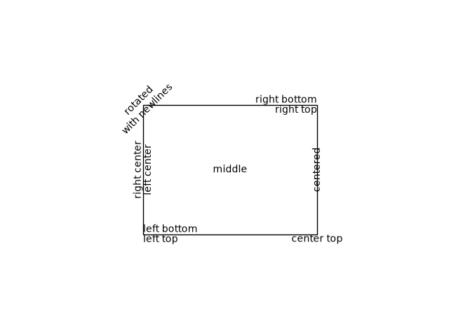
text_labels_and_annotations/text_commands
===============
Source
"""
===============
Text properties
===============
Plotting text of many different kinds.
.. redirect-from:: /gallery/pyplots/text_commands
"""
import matplotlib.pyplot as plt
fig = plt.figure()
fig.suptitle('bold figure suptitle', fontsize=14, fontweight='bold')
ax = fig.add_subplot()
fig.subplots_adjust(top=0.85)
ax.set_title('axes title')
ax.set_xlabel('xlabel')
ax.set_ylabel('ylabel')
ax.text(3, 8, 'boxed italics text in data coords', style='italic',
bbox={'facecolor': 'red', 'alpha': 0.5, 'pad': 10})
ax.text(2, 6, r'an equation: $E=mc^2$', fontsize=15)
ax.text(3, 2, 'Unicode: Institut f\374r Festk\366rperphysik')
ax.text(0.95, 0.01, 'colored text in axes coords',
verticalalignment='bottom', horizontalalignment='right',
transform=ax.transAxes,
color='green', fontsize=15)
ax.plot([2], [1], 'o')
ax.annotate('annotate', xy=(2, 1), xytext=(3, 4),
arrowprops=dict(facecolor='black', shrink=0.05))
ax.set(xlim=(0, 10), ylim=(0, 10))
plt.show()
# %%
#
# .. admonition:: References
#
# The use of the following functions, methods, classes and modules is shown
# in this example:
#
# - `matplotlib.figure.Figure.suptitle`
# - `matplotlib.figure.Figure.add_subplot`
# - `matplotlib.figure.Figure.subplots_adjust`
# - `matplotlib.axes.Axes.set_title`
# - `matplotlib.axes.Axes.set_xlabel`
# - `matplotlib.axes.Axes.set_ylabel`
# - `matplotlib.axes.Axes.text`
# - `matplotlib.axes.Axes.annotate`
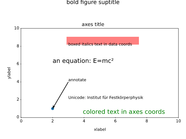
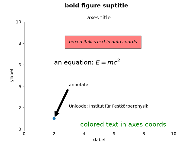
text_labels_and_annotations/text_fontdict
=======================================================
Source
"""
=======================================================
Controlling style of text and labels using a dictionary
=======================================================
This example shows how to share parameters across many text objects and labels
by creating a dictionary of options passed across several functions.
"""
import matplotlib.pyplot as plt
import numpy as np
font = {'family': 'serif',
'color': 'darkred',
'weight': 'normal',
'size': 16,
}
x = np.linspace(0.0, 5.0, 100)
y = np.cos(2*np.pi*x) * np.exp(-x)
plt.plot(x, y, 'k')
plt.title('Damped exponential decay', fontdict=font)
plt.text(2, 0.65, r'$\cos(2 \pi t) \exp(-t)$', fontdict=font)
plt.xlabel('time (s)', fontdict=font)
plt.ylabel('voltage (mV)', fontdict=font)
# Tweak spacing to prevent clipping of ylabel
plt.subplots_adjust(left=0.15)
plt.show()
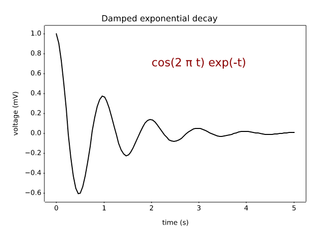
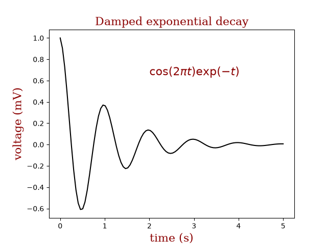
text_labels_and_annotations/text_rotation_relative_to_line
=======================================
Source
"""
=======================================
Text rotation angle in data coordinates
=======================================
Text objects in matplotlib are normally rotated with respect to the
screen coordinate system (i.e., 45 degrees rotation plots text along a
line that is in between horizontal and vertical no matter how the axes
are changed). However, at times one wants to rotate text with respect
to something on the plot. In this case, the correct angle won't be
the angle of that object in the plot coordinate system, but the angle
that that object APPEARS in the screen coordinate system. This angle
can be determined automatically by setting the parameter
*transform_rotates_text*, as shown in the example below.
"""
import matplotlib.pyplot as plt
fig, ax = plt.subplots()
# Plot diagonal line (45 degrees in data coordinates)
ax.plot(range(0, 8), range(0, 8))
ax.set_xlim([-10, 10])
# Plot text
ax.text(-8, 0, 'text 45° in screen coordinates', fontsize=18,
rotation=45, rotation_mode='anchor')
ax.text(0, 0, 'text 45° in data coordinates', fontsize=18,
rotation=45, rotation_mode='anchor',
transform_rotates_text=True)
plt.show()
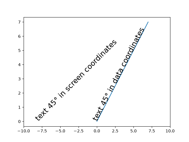
text_labels_and_annotations/titles_demo
=================
Source
"""
=================
Title positioning
=================
Matplotlib can display plot titles centered, flush with the left side of
a set of Axes, and flush with the right side of a set of Axes.
"""
import matplotlib.pyplot as plt
plt.plot(range(10))
plt.title('Center Title')
plt.title('Left Title', loc='left')
plt.title('Right Title', loc='right')
plt.show()
# %%
# The vertical position is automatically chosen to avoid decorations
# (i.e. labels and ticks) on the topmost x-axis:
fig, axs = plt.subplots(1, 2, layout='constrained')
ax = axs[0]
ax.plot(range(10))
ax.xaxis.set_label_position('top')
ax.set_xlabel('X-label')
ax.set_title('Center Title')
ax = axs[1]
ax.plot(range(10))
ax.xaxis.set_label_position('top')
ax.xaxis.tick_top()
ax.set_xlabel('X-label')
ax.set_title('Center Title')
plt.show()
# %%
# Automatic positioning can be turned off by manually specifying the *y*
# keyword argument for the title or setting :rc:`axes.titley` in the rcParams.
fig, axs = plt.subplots(1, 2, layout='constrained')
ax = axs[0]
ax.plot(range(10))
ax.xaxis.set_label_position('top')
ax.set_xlabel('X-label')
ax.set_title('Manual y', y=1.0, pad=-14)
plt.rcParams['axes.titley'] = 1.0 # y is in axes-relative coordinates.
plt.rcParams['axes.titlepad'] = -14 # pad is in points...
ax = axs[1]
ax.plot(range(10))
ax.set_xlabel('X-label')
ax.set_title('rcParam y')
plt.show()
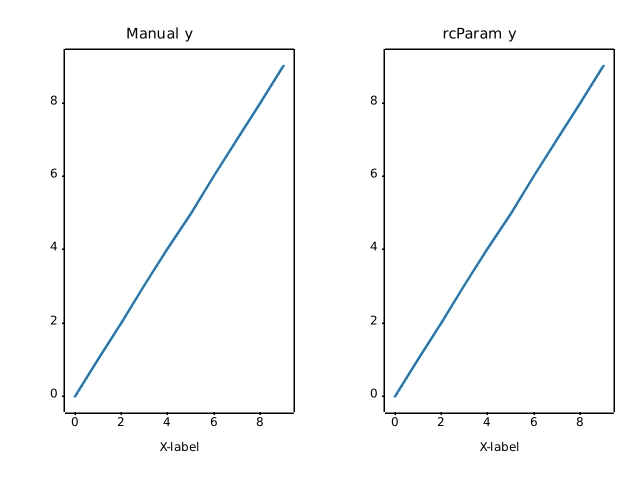
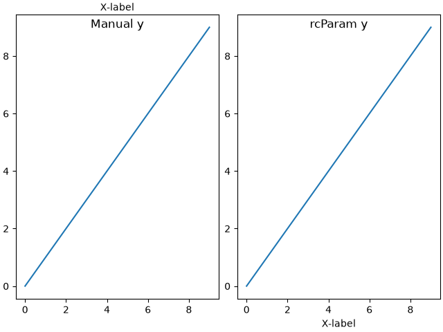
text_labels_and_annotations/unicode_minus
=============
Source
"""
=============
Unicode minus
=============
By default, tick labels at negative values are rendered using a `Unicode
minus`__ (U+2212) rather than an ASCII hyphen (U+002D). This can be controlled
by setting :rc:`axes.unicode_minus`.
__ https://en.wikipedia.org/wiki/Plus_and_minus_signs#Character_codes
The replacement is performed at draw time of the tick labels (usually during a
`.pyplot.show()` or `.pyplot.savefig()` call). Therefore, all tick labels of
the figure follow the same setting and we cannot demonstrate both glyphs on
real tick labels of the same figure simultaneously.
Instead, this example simply showcases the difference between the two glyphs
in a magnified font.
"""
import matplotlib.pyplot as plt
fig = plt.figure(figsize=(4, 2))
fig.text(.15, .6, "Unicode minus:", fontsize=20)
fig.text(.85, .6, "\N{MINUS SIGN}1", ha='right', fontsize=20)
fig.text(.15, .3, "ASCII hyphen:", fontsize=20)
fig.text(.85, .3, "-1", ha='right', fontsize=20)
plt.show()
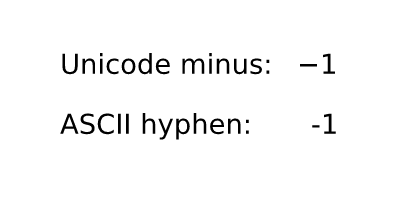
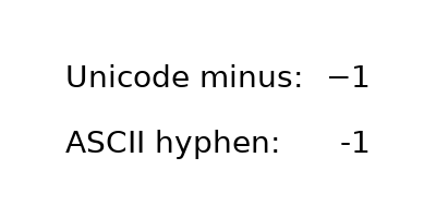
text_labels_and_annotations/usetex_baseline_test
====================
Source
"""
====================
Usetex text baseline
====================
Comparison of text baselines computed for mathtext and usetex.
"""
import matplotlib.pyplot as plt
plt.rcParams.update({"mathtext.fontset": "cm", "mathtext.rm": "serif"})
axs = plt.figure(figsize=(2 * 3, 6.5)).subplots(1, 2)
for ax, usetex in zip(axs, [False, True]):
ax.axvline(0, color="r")
test_strings = ["lg", r"$\frac{1}{2}\pi$", r"$p^{3^A}$", r"$p_{3_2}$"]
for i, s in enumerate(test_strings):
ax.axhline(i, color="r")
ax.text(0., 3 - i, s,
usetex=usetex,
verticalalignment="baseline",
size=50,
bbox=dict(pad=0, ec="k", fc="none"))
ax.set(xlim=(-0.1, 1.1), ylim=(-.8, 3.9), xticks=[], yticks=[],
title=f"usetex={usetex}\n")
plt.show()
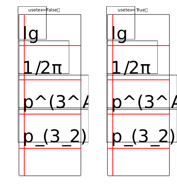
RuntimeError: Failed to process string with tex because latex could not be found
text_labels_and_annotations/usetex_fonteffects
===================
Source
"""
===================
Usetex font effects
===================
This script demonstrates that font effects specified in your pdftex.map
are now supported in usetex mode.
"""
import matplotlib.pyplot as plt
def setfont(font):
return rf'\font\a {font} at 14pt\a '
fig = plt.figure()
for y, font, text in zip(
range(5),
['ptmr8r', 'ptmri8r', 'ptmro8r', 'ptmr8rn', 'ptmrr8re'],
[f'Nimbus Roman No9 L {x}'
for x in ['', 'Italics (real italics for comparison)',
'(slanted)', '(condensed)', '(extended)']],
):
fig.text(.1, 1 - (y + 1) / 6, setfont(font) + text, usetex=True)
fig.suptitle('Usetex font effects')
# Would also work if saving to pdf.
plt.show()
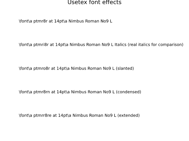
RuntimeError: Failed to process string with tex because latex could not be found
text_labels_and_annotations/watermark_text
==============
Source
"""
==============
Text watermark
==============
A watermark effect can be achieved by drawing a semi-transparent text.
"""
import matplotlib.pyplot as plt
import numpy as np
# Fixing random state for reproducibility
np.random.seed(19680801)
fig, ax = plt.subplots()
ax.plot(np.random.rand(20), '-o', ms=20, lw=2, alpha=0.7, mfc='orange')
ax.grid()
ax.text(0.5, 0.5, 'created with matplotlib', transform=ax.transAxes,
fontsize=40, color='gray', alpha=0.5,
ha='center', va='center', rotation=30)
plt.show()
# %%
#
# .. admonition:: References
#
# The use of the following functions, methods, classes and modules is shown
# in this example:
#
# - `matplotlib.figure.Figure.text`
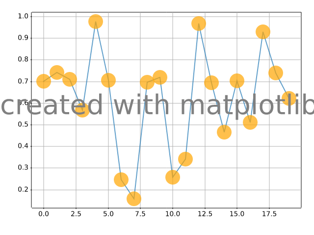
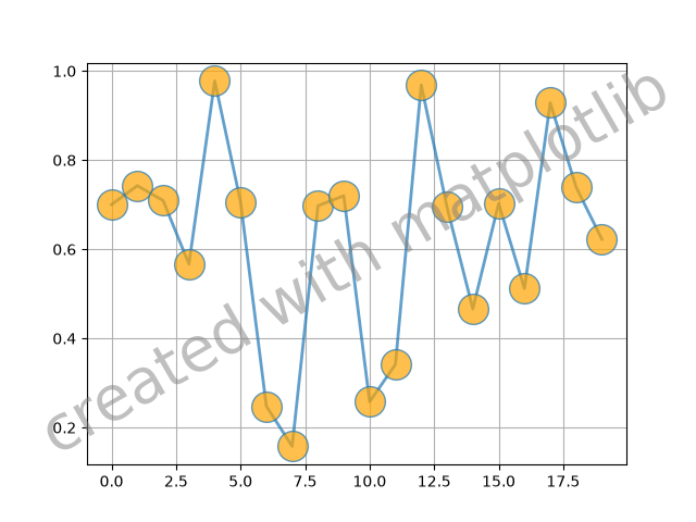
ticks/align_ticklabels
=================
Source
"""
=================
Align tick labels
=================
By default, tick labels are aligned towards the axis. This means the set of
*y* tick labels appear right-aligned. Because the alignment reference point
is on the axis, left-aligned tick labels would overlap the plotting area.
To achieve a good-looking left-alignment, you have to additionally increase
the padding.
"""
import matplotlib.pyplot as plt
population = {
"Sydney": 5.2,
"Mexico City": 8.8,
"São Paulo": 12.2,
"Istanbul": 15.9,
"Lagos": 15.9,
"Shanghai": 21.9,
}
fig, ax = plt.subplots(layout="constrained")
ax.barh(population.keys(), population.values())
ax.set_xlabel('Population (in millions)')
# left-align all ticklabels
for ticklabel in ax.get_yticklabels():
ticklabel.set_horizontalalignment("left")
# increase padding
ax.tick_params("y", pad=70)
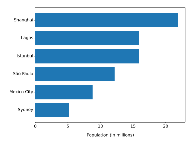
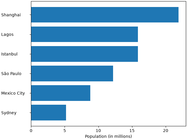
ticks/auto_ticks
====================================
Source
""" ==================================== Automatically setting tick positions ==================================== Setting the behavior of tick auto-placement. By default, Matplotlib will choose the number of ticks and tick positions so that there is a reasonable number of ticks on the axis and they are located at "round" numbers. As a result, there may be no ticks on the edges of the plot. """ import matplotlib.pyplot as plt import numpy as np np.random.seed(19680801) fig, ax = plt.subplots() dots = np.linspace(0.3, 1.2, 10) X, Y = np.meshgrid(dots, dots) x, y = X.ravel(), Y.ravel() ax.scatter(x, y, c=x+y) plt.show() # %% # If you want to keep ticks at round numbers, and also have ticks at the edges # you can switch :rc:`axes.autolimit_mode` to 'round_numbers'. This expands the # axis limits to the next round number. plt.rcParams['axes.autolimit_mode'] = 'round_numbers' # Note: The limits are calculated at draw-time. Therefore, when using # :rc:`axes.autolimit_mode` in a context manager, it is important that # the ``show()`` command is within the context. fig, ax = plt.subplots() ax.scatter(x, y, c=x+y) plt.show() # %% # The round numbers autolimit_mode is still respected if you set an additional # margin around the data using `.Axes.set_xmargin` / `.Axes.set_ymargin`: fig, ax = plt.subplots() ax.scatter(x, y, c=x+y) ax.set_xmargin(0.8) plt.show()
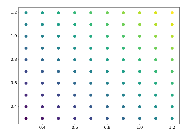
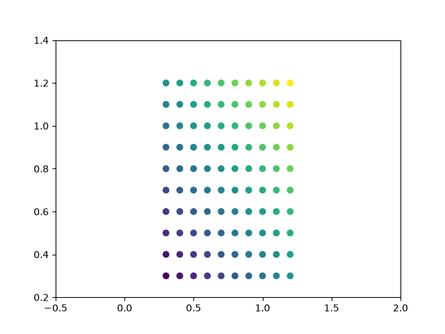
ticks/centered_ticklabels
===========================
Source
"""
===========================
Center labels between ticks
===========================
Tick labels are aligned relative to their associated tick, and are by default
centered.
However, there is no direct way to center the labels between ticks. To fake
this behavior, one can place a minor tick in between the major ticks. Then
label the minor tick, and hide the minor tick lines and the major tick labels.
Here is an example that labels the months, centered between the ticks.
"""
import matplotlib.pyplot as plt
import matplotlib.cbook as cbook
import matplotlib.dates as dates
import matplotlib.ticker as ticker
# Load some financial data; Google's stock price
r = cbook.get_sample_data('goog.npz')['price_data']
r = r[-250:] # get the last 250 days
fig, ax = plt.subplots()
ax.plot(r["date"], r["adj_close"])
ax.xaxis.set_major_locator(dates.MonthLocator())
# 16 is a slight approximation since months differ in number of days.
ax.xaxis.set_minor_locator(dates.MonthLocator(bymonthday=16))
# The NullFormatter removes the major tick labels
ax.xaxis.set_major_formatter(ticker.NullFormatter())
ax.xaxis.set_minor_formatter(dates.DateFormatter('%b'))
# Remove the minor tick lines
ax.tick_params(axis='x', which='minor', tick1On=False, tick2On=False)
imid = len(r) // 2
ax.set_xlabel(str(r["date"][imid].item().year))
plt.show()
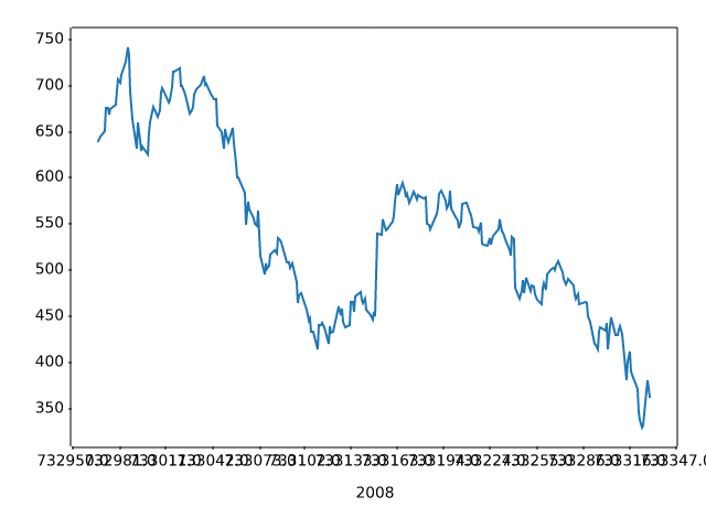
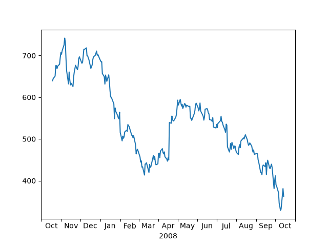
ticks/colorbar_tick_labelling_demo
=======================
Source
"""
=======================
Colorbar Tick labelling
=======================
Vertical colorbars have ticks, tick labels, and labels visible on the *y* axis,
horizontal colorbars on the *x* axis. The ``ticks`` parameter can be used to
set the ticks and the ``format`` parameter can be used to format the tick labels
of the visible colorbar Axes. For further adjustments, the ``yaxis`` or
``xaxis`` Axes of the colorbar can be retrieved using its ``ax`` property.
"""
import matplotlib.pyplot as plt
import numpy as np
import matplotlib.ticker as mticker
# Fixing random state for reproducibility
rng = np.random.default_rng(seed=19680801)
# %%
# Make plot with vertical (default) colorbar
fig, ax = plt.subplots()
data = rng.standard_normal((250, 250))
cax = ax.imshow(data, vmin=-1, vmax=1, cmap='coolwarm')
ax.set_title('Gaussian noise with vertical colorbar')
# Add colorbar, make sure to specify tick locations to match desired ticklabels
cbar = fig.colorbar(cax,
ticks=[-1, 0, 1],
format=mticker.FixedFormatter(['< -1', '0', '> 1']),
extend='both'
)
labels = cbar.ax.get_yticklabels()
labels[0].set_verticalalignment('top')
labels[-1].set_verticalalignment('bottom')
# %%
# Make plot with horizontal colorbar
fig, ax = plt.subplots()
data = np.clip(data, -1, 1)
cax = ax.imshow(data, cmap='afmhot')
ax.set_title('Gaussian noise with horizontal colorbar')
# Add colorbar and adjust ticks afterwards
cbar = fig.colorbar(cax, orientation='horizontal')
cbar.set_ticks(ticks=[-1, 0, 1], labels=['Low', 'Medium', 'High'])
plt.show()
# %%
#
# .. admonition:: References
#
# The use of the following functions, methods, classes and modules is shown
# in this example:
#
# - `matplotlib.colorbar.Colorbar.set_ticks`
# - `matplotlib.figure.Figure.colorbar` / `matplotlib.pyplot.colorbar`
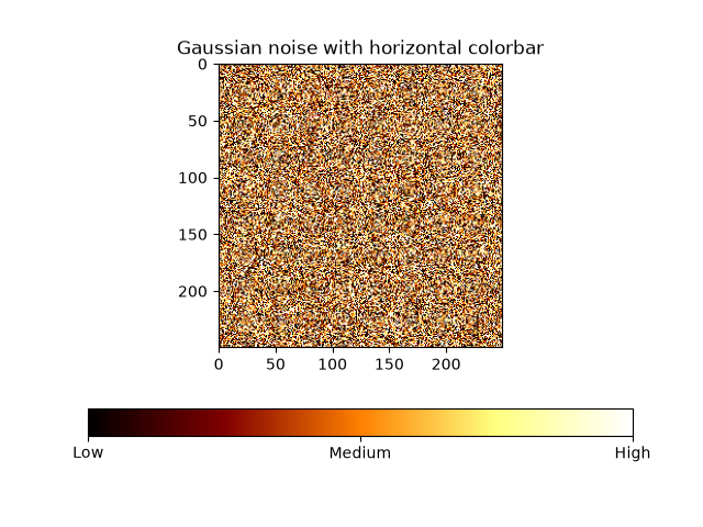
ticks/custom_ticker1
=============
Source
"""
=============
Custom Ticker
=============
The :mod:`matplotlib.ticker` module defines many preset tickers, but was
primarily designed for extensibility, i.e., to support user customized ticking.
In this example, a user defined function is used to format the ticks in
millions of dollars on the y-axis.
"""
import matplotlib.pyplot as plt
def millions(x, pos):
"""The two arguments are the value and tick position."""
return f'${x*1e-6:1.1f}M'
fig, ax = plt.subplots()
# set_major_formatter internally creates a FuncFormatter from the callable.
ax.yaxis.set_major_formatter(millions)
money = [1.5e5, 2.5e6, 5.5e6, 2.0e7]
ax.bar(['Bill', 'Fred', 'Mary', 'Sue'], money)
plt.show()
# %%
#
# .. admonition:: References
#
# The use of the following functions, methods, classes and modules is shown
# in this example:
#
# - `matplotlib.axis.Axis.set_major_formatter`
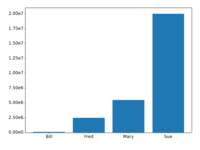
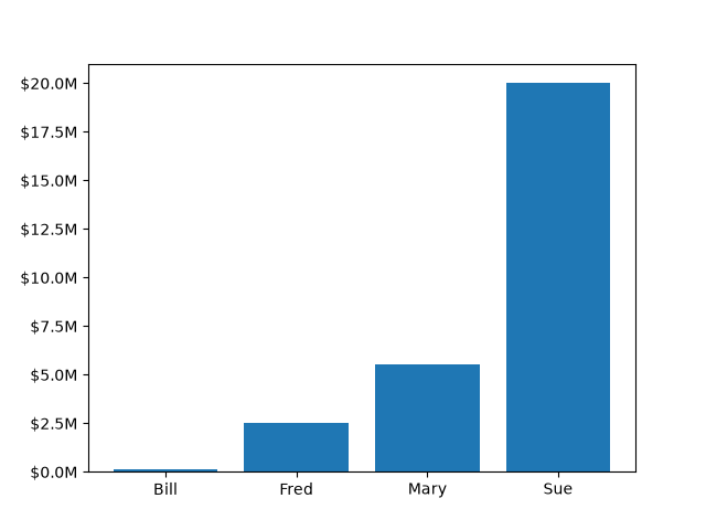
ticks/date
================
Source
"""
================
Date tick labels
================
Matplotlib date plotting is done by converting date instances into
days since an epoch (by default 1970-01-01T00:00:00). The
:mod:`matplotlib.dates` module provides the converter functions `.date2num`
and `.num2date` that convert `datetime.datetime` and `numpy.datetime64`
objects to and from Matplotlib's internal representation. These data
types are registered with the unit conversion mechanism described in
:mod:`matplotlib.units`, so the conversion happens automatically for the user.
The registration process also sets the default tick ``locator`` and
``formatter`` for the axis to be `~.matplotlib.dates.AutoDateLocator` and
`~.matplotlib.dates.AutoDateFormatter`.
An alternative formatter is the `~.dates.ConciseDateFormatter`,
used in the second ``Axes`` below (see
:doc:`/gallery/ticks/date_concise_formatter`), which often removes the need to
rotate the tick labels. The last ``Axes`` formats the dates manually, using
`~.dates.DateFormatter` to format the dates using the format strings documented
at `datetime.date.strftime`.
.. redirect-from:: /gallery/text_labels_and_annotations/date
"""
import matplotlib.pyplot as plt
import matplotlib.cbook as cbook
import matplotlib.dates as mdates
# Load a numpy record array from yahoo csv data with fields date, open, high,
# low, close, volume, adj_close from the mpl-data/sample_data directory. The
# record array stores the date as an np.datetime64 with a day unit ('D') in
# the date column.
data = cbook.get_sample_data('goog.npz')['price_data']
fig, axs = plt.subplots(3, 1, figsize=(6.4, 7), layout='constrained')
# common to all three:
for ax in axs:
ax.plot('date', 'adj_close', data=data)
# Major ticks every half year, minor ticks every month,
ax.xaxis.set_major_locator(mdates.MonthLocator(bymonth=(1, 7)))
ax.xaxis.set_minor_locator(mdates.MonthLocator())
ax.grid(True)
ax.set_ylabel(r'Price [\$]')
# different formats:
ax = axs[0]
ax.set_title('DefaultFormatter', loc='left', y=0.85, x=0.02, fontsize='medium')
ax = axs[1]
ax.set_title('ConciseFormatter', loc='left', y=0.85, x=0.02, fontsize='medium')
ax.xaxis.set_major_formatter(
mdates.ConciseDateFormatter(ax.xaxis.get_major_locator()))
ax = axs[2]
ax.set_title('Manual DateFormatter', loc='left', y=0.85, x=0.02,
fontsize='medium')
# Text in the x-axis will be displayed in 'YYYY-mm' format.
ax.xaxis.set_major_formatter(mdates.DateFormatter('%Y-%b'))
# Rotates and right-aligns the x labels so they don't crowd each other.
ax.xaxis.set_tick_params(rotation=30, rotation_mode='xtick')
plt.show()
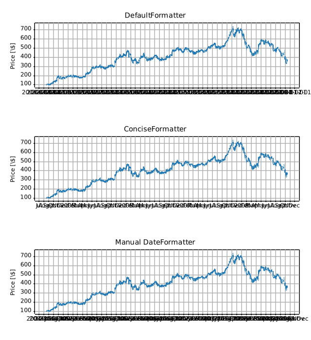
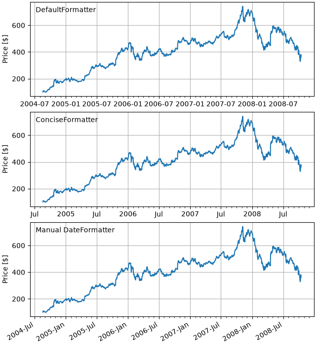
ticks/date_concise_formatter
.. _date_concise_formatter:
Source
"""
.. _date_concise_formatter:
============================================
Format date ticks using ConciseDateFormatter
============================================
Finding good tick values and formatting the ticks for an axis that
has date data is often a challenge. `~.dates.ConciseDateFormatter` is
meant to improve the strings chosen for the ticklabels, and to minimize
the strings used in those tick labels as much as possible.
.. note::
This formatter is a candidate to become the default date tick formatter
in future versions of Matplotlib. Please report any issues or
suggestions for improvement to the GitHub repository or mailing list.
"""
import datetime
import matplotlib.pyplot as plt
import numpy as np
import matplotlib.dates as mdates
# %%
# First, the default formatter.
base = datetime.datetime(2005, 2, 1)
dates = [base + datetime.timedelta(hours=(2 * i)) for i in range(732)]
N = len(dates)
np.random.seed(19680801)
y = np.cumsum(np.random.randn(N))
fig, axs = plt.subplots(3, 1, layout='constrained', figsize=(6, 6))
lims = [(np.datetime64('2005-02'), np.datetime64('2005-04')),
(np.datetime64('2005-02-03'), np.datetime64('2005-02-15')),
(np.datetime64('2005-02-03 11:00'), np.datetime64('2005-02-04 13:20'))]
for nn, ax in enumerate(axs):
ax.plot(dates, y)
ax.set_xlim(lims[nn])
ax.tick_params(axis='x', rotation=40, rotation_mode='xtick')
axs[0].set_title('Default Date Formatter')
plt.show()
# %%
# The default date formatter is quite verbose, so we have the option of
# using `~.dates.ConciseDateFormatter`, as shown below. Note that
# for this example the labels do not need to be rotated as they do for the
# default formatter because the labels are as small as possible.
fig, axs = plt.subplots(3, 1, layout='constrained', figsize=(6, 6))
for nn, ax in enumerate(axs):
locator = mdates.AutoDateLocator(minticks=3, maxticks=7)
formatter = mdates.ConciseDateFormatter(locator)
ax.xaxis.set_major_locator(locator)
ax.xaxis.set_major_formatter(formatter)
ax.plot(dates, y)
ax.set_xlim(lims[nn])
axs[0].set_title('Concise Date Formatter')
plt.show()
# %%
# If all calls to axes that have dates are to be made using this converter,
# it is probably most convenient to use the units registry where you do
# imports:
import matplotlib.units as munits
converter = mdates.ConciseDateConverter()
munits.registry[np.datetime64] = converter
munits.registry[datetime.date] = converter
munits.registry[datetime.datetime] = converter
fig, axs = plt.subplots(3, 1, figsize=(6, 6), layout='constrained')
for nn, ax in enumerate(axs):
ax.plot(dates, y)
ax.set_xlim(lims[nn])
axs[0].set_title('Concise Date Formatter')
plt.show()
# %%
# Localization of date formats
# ============================
#
# Dates formats can be localized if the default formats are not desirable by
# manipulating one of three lists of strings.
#
# The ``formatter.formats`` list of formats is for the normal tick labels,
# There are six levels: years, months, days, hours, minutes, seconds.
# The ``formatter.offset_formats`` is how the "offset" string on the right
# of the axis is formatted. This is usually much more verbose than the tick
# labels. Finally, the ``formatter.zero_formats`` are the formats of the
# ticks that are "zeros". These are tick values that are either the first of
# the year, month, or day of month, or the zeroth hour, minute, or second.
# These are usually the same as the format of
# the ticks a level above. For example if the axis limits mean the ticks are
# mostly days, then we label 1 Mar 2005 simply with a "Mar". If the axis
# limits are mostly hours, we label Feb 4 00:00 as simply "Feb-4".
#
# Note that these format lists can also be passed to `.ConciseDateFormatter`
# as optional keyword arguments.
#
# Here we modify the labels to be "day month year", instead of the ISO
# "year month day":
fig, axs = plt.subplots(3, 1, layout='constrained', figsize=(6, 6))
for nn, ax in enumerate(axs):
locator = mdates.AutoDateLocator()
formatter = mdates.ConciseDateFormatter(locator)
formatter.formats = ['%y', # ticks are mostly years
'%b', # ticks are mostly months
'%d', # ticks are mostly days
'%H:%M', # hrs
'%H:%M', # min
'%S.%f', ] # secs
# these are mostly just the level above...
formatter.zero_formats = [''] + formatter.formats[:-1]
# ...except for ticks that are mostly hours, then it is nice to have
# month-day:
formatter.zero_formats[3] = '%d-%b'
formatter.offset_formats = ['',
'%Y',
'%b %Y',
'%d %b %Y',
'%d %b %Y',
'%d %b %Y %H:%M', ]
ax.xaxis.set_major_locator(locator)
ax.xaxis.set_major_formatter(formatter)
ax.plot(dates, y)
ax.set_xlim(lims[nn])
axs[0].set_title('Concise Date Formatter')
plt.show()
# %%
# Registering a converter with localization
# =========================================
#
# `.ConciseDateFormatter` doesn't have rcParams entries, but localization can
# be accomplished by passing keyword arguments to `.ConciseDateConverter` and
# registering the datatypes you will use with the units registry:
import datetime
formats = ['%y', # ticks are mostly years
'%b', # ticks are mostly months
'%d', # ticks are mostly days
'%H:%M', # hrs
'%H:%M', # min
'%S.%f', ] # secs
# these can be the same, except offset by one level....
zero_formats = [''] + formats[:-1]
# ...except for ticks that are mostly hours, then it's nice to have month-day
zero_formats[3] = '%d-%b'
offset_formats = ['',
'%Y',
'%b %Y',
'%d %b %Y',
'%d %b %Y',
'%d %b %Y %H:%M', ]
converter = mdates.ConciseDateConverter(
formats=formats, zero_formats=zero_formats, offset_formats=offset_formats)
munits.registry[np.datetime64] = converter
munits.registry[datetime.date] = converter
munits.registry[datetime.datetime] = converter
fig, axs = plt.subplots(3, 1, layout='constrained', figsize=(6, 6))
for nn, ax in enumerate(axs):
ax.plot(dates, y)
ax.set_xlim(lims[nn])
axs[0].set_title('Concise Date Formatter registered non-default')
plt.show()
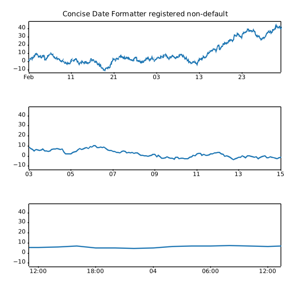
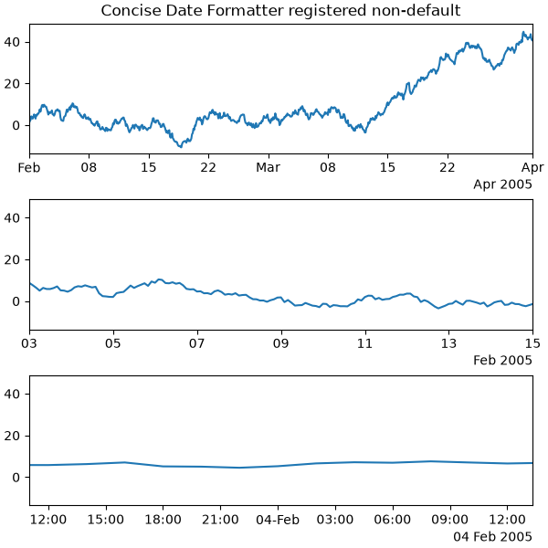
ticks/date_demo_convert
===================
Source
"""
===================
Date converter demo
===================
"""
import datetime
import matplotlib.pyplot as plt
import numpy as np
from matplotlib.dates import DateFormatter, DayLocator, HourLocator, drange
date1 = datetime.datetime(2000, 3, 2)
date2 = datetime.datetime(2000, 3, 6)
delta = datetime.timedelta(hours=6)
dates = drange(date1, date2, delta)
y = np.arange(len(dates))
fig, ax = plt.subplots()
ax.plot(dates, y**2, 'o')
# This is superfluous, since the autoscaler should get it right, but
# use date2num and num2date to convert between dates and floats if
# you want; both date2num and num2date convert an instance or sequence.
ax.set_xlim(dates[0], dates[-1])
# The hour locator takes the hour or sequence of hours you want to
# tick, not the base multiple.
ax.xaxis.set_major_locator(DayLocator())
ax.xaxis.set_minor_locator(HourLocator(range(0, 25, 6)))
ax.xaxis.set_major_formatter(DateFormatter('%Y-%m-%d'))
ax.fmt_xdata = DateFormatter('%Y-%m-%d %H:%M:%S')
fig.autofmt_xdate()
plt.show()
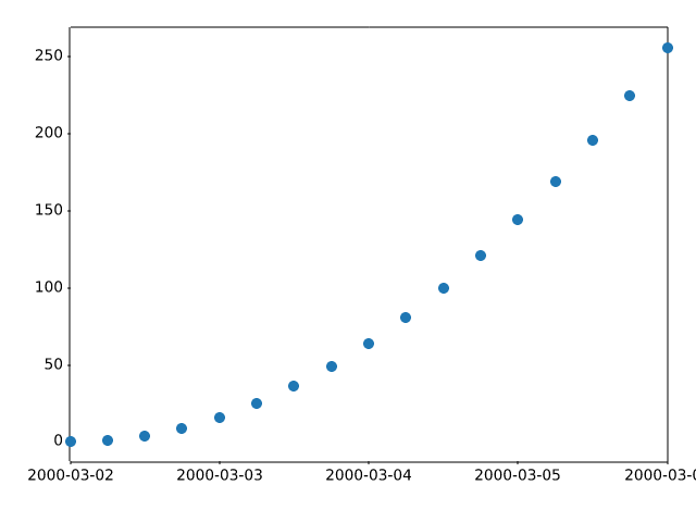
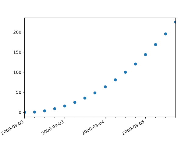
ticks/date_demo_rrule
=========================================
Source
"""
=========================================
Placing date ticks using recurrence rules
=========================================
The `iCalender RFC`_ specifies *recurrence rules* (rrules), that define
date sequences. You can use rrules in Matplotlib to place date ticks.
This example sets custom date ticks on every 5th easter.
See https://dateutil.readthedocs.io/en/stable/rrule.html for help with rrules.
.. _iCalender RFC: https://tools.ietf.org/html/rfc5545
"""
import datetime
import matplotlib.pyplot as plt
import numpy as np
from matplotlib.dates import YEARLY, DateFormatter, RRuleLocator, drange, rrulewrapper
# Fixing random state for reproducibility
np.random.seed(19680801)
# tick every 5th easter
rule = rrulewrapper(YEARLY, byeaster=1, interval=5)
loc = RRuleLocator(rule)
formatter = DateFormatter('%m/%d/%y')
date1 = datetime.date(1952, 1, 1)
date2 = datetime.date(2004, 4, 12)
delta = datetime.timedelta(days=100)
dates = drange(date1, date2, delta)
s = np.random.rand(len(dates)) # make up some random y values
fig, ax = plt.subplots()
plt.plot(dates, s, 'o')
ax.xaxis.set_major_locator(loc)
ax.xaxis.set_major_formatter(formatter)
ax.xaxis.set_tick_params(rotation=30, labelsize=10)
plt.show()
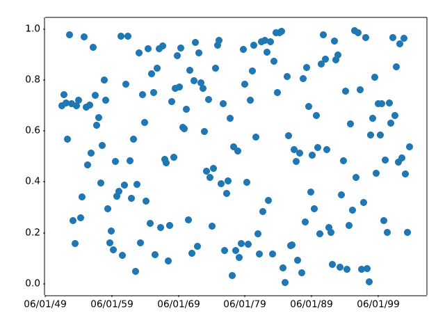
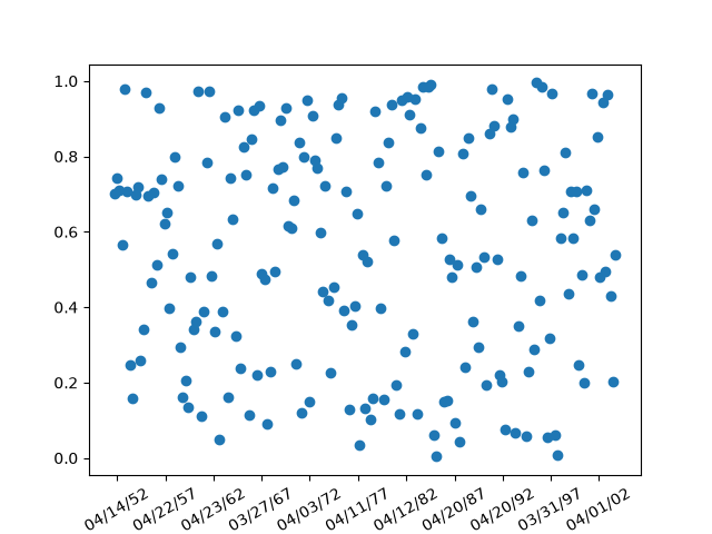
ticks/date_formatters_locators
.. _date_formatters_locators:
Source
"""
.. _date_formatters_locators:
=================================
Date tick locators and formatters
=================================
This example illustrates the usage and effect of the various date locators and
formatters.
"""
import matplotlib.pyplot as plt
import numpy as np
# While these appear unused directly, they are used from eval'd strings.
from matplotlib.dates import (FR, MO, MONTHLY, SA, SU, TH, TU, WE, AutoDateFormatter,
AutoDateLocator, ConciseDateFormatter, DateFormatter,
DayLocator, HourLocator, MicrosecondLocator,
MinuteLocator, MonthLocator, RRuleLocator, SecondLocator,
WeekdayLocator, YearLocator, rrulewrapper)
import matplotlib.ticker as ticker
def plot_axis(ax, locator=None, xmax='2002-02-01', fmt=None, formatter=None):
"""Set up common parameters for the Axes in the example."""
ax.spines[['left', 'right', 'top']].set_visible(False)
ax.yaxis.set_major_locator(ticker.NullLocator())
ax.tick_params(which='major', width=1.00, length=5)
ax.tick_params(which='minor', width=0.75, length=2.5)
ax.set_xlim(np.datetime64('2000-02-01'), np.datetime64(xmax))
if locator:
ax.xaxis.set_major_locator(eval(locator))
ax.xaxis.set_major_formatter(DateFormatter(fmt))
else:
ax.xaxis.set_major_formatter(eval(formatter))
ax.text(0.0, 0.2, locator or formatter, transform=ax.transAxes,
fontsize=14, fontname='Monospace', color='tab:blue')
# %%
# :ref:`date-locators`
# --------------------
locators = [
# locator as str, xmax, fmt
('AutoDateLocator(maxticks=8)', '2003-02-01', '%Y-%m'),
('YearLocator(month=4)', '2003-02-01', '%Y-%m'),
('MonthLocator(bymonth=[4, 8, 12])', '2003-02-01', '%Y-%m'),
('DayLocator(interval=180)', '2003-02-01', '%Y-%m-%d'),
('WeekdayLocator(byweekday=SU, interval=4)', '2000-07-01', '%a %Y-%m-%d'),
('HourLocator(byhour=range(0, 24, 6))', '2000-02-04', '%H h'),
('MinuteLocator(interval=15)', '2000-02-01 02:00', '%H:%M'),
('SecondLocator(bysecond=(0, 30))', '2000-02-01 00:02', '%H:%M:%S'),
('MicrosecondLocator(interval=1000)', '2000-02-01 00:00:00.005', '%S.%f'),
('RRuleLocator(rrulewrapper(freq=MONTHLY, \nbyweekday=(MO, TU, WE, TH, FR), '
'bysetpos=-1))', '2000-07-01', '%Y-%m-%d'),
]
fig, axs = plt.subplots(len(locators), 1, figsize=(8, len(locators) * .8),
layout='constrained')
fig.suptitle('Date Locators')
for ax, (locator, xmax, fmt) in zip(axs, locators):
plot_axis(ax, locator, xmax, fmt)
# %%
# :ref:`date-formatters`
# ----------------------
formatters = [
'AutoDateFormatter(ax.xaxis.get_major_locator())',
'ConciseDateFormatter(ax.xaxis.get_major_locator())',
'DateFormatter("%b %Y")',
]
fig, axs = plt.subplots(len(formatters), 1, figsize=(8, len(formatters) * .8),
layout='constrained')
fig.suptitle('Date Formatters')
for ax, fmt in zip(axs, formatters):
plot_axis(ax, formatter=fmt)
# %%
#
# .. admonition:: References
#
# The use of the following functions, methods, classes and modules is shown
# in this example:
#
# - `matplotlib.dates.AutoDateLocator`
# - `matplotlib.dates.YearLocator`
# - `matplotlib.dates.MonthLocator`
# - `matplotlib.dates.DayLocator`
# - `matplotlib.dates.WeekdayLocator`
# - `matplotlib.dates.HourLocator`
# - `matplotlib.dates.MinuteLocator`
# - `matplotlib.dates.SecondLocator`
# - `matplotlib.dates.MicrosecondLocator`
# - `matplotlib.dates.RRuleLocator`
# - `matplotlib.dates.rrulewrapper`
# - `matplotlib.dates.DateFormatter`
# - `matplotlib.dates.AutoDateFormatter`
# - `matplotlib.dates.ConciseDateFormatter`
#
# .. tags:: component: ticks, purpose: reference
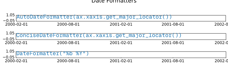
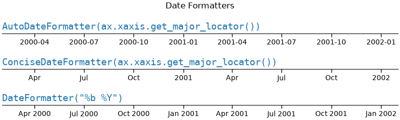
ticks/date_index_formatter
=====================================
Source
"""
=====================================
Custom tick formatter for time series
=====================================
.. redirect-from:: /gallery/text_labels_and_annotations/date_index_formatter
.. redirect-from:: /gallery/ticks/date_index_formatter2
When plotting daily data, e.g., financial time series, one often wants
to leave out days on which there is no data, for instance weekends, so that
the data are plotted at regular intervals without extra spaces for the days
with no data.
The example shows how to use an 'index formatter' to achieve the desired plot.
"""
import matplotlib.pyplot as plt
import numpy as np
import matplotlib.cbook as cbook
from matplotlib.dates import DateFormatter, DayLocator
import matplotlib.lines as ml
from matplotlib.ticker import Formatter
# Load a structured numpy array from yahoo csv data with fields date, open, high,
# low, close, volume, adj_close from the mpl-data/sample_data directory. The
# record array stores the date as an np.datetime64 with a day unit ('D') in
# the date column (``r['date']``).
r = cbook.get_sample_data('goog.npz')['price_data']
r = r[:9] # get the first 9 days
fig, (ax1, ax2) = plt.subplots(nrows=2, figsize=(6, 6), layout='constrained')
fig.get_layout_engine().set(hspace=0.15)
# First we'll do it the default way, with gaps on weekends
ax1.plot(r["date"], r["adj_close"], 'o-')
# Highlight gaps in daily data
gaps = np.flatnonzero(np.diff(r["date"]) > np.timedelta64(1, 'D'))
for gap in r[['date', 'adj_close']][np.stack((gaps, gaps + 1)).T]:
ax1.plot(gap['date'], gap['adj_close'], 'w--', lw=2)
ax1.legend(handles=[ml.Line2D([], [], ls='--', label='Gaps in daily data')])
ax1.set_title("Plot y at x Coordinates")
ax1.xaxis.set_major_locator(DayLocator())
ax1.xaxis.set_major_formatter(DateFormatter('%a'))
# Next we'll write a custom index formatter. Below we will plot
# the data against an index that goes from 0, 1, ... len(data). Instead of
# formatting the tick marks as integers, we format as times.
def format_date(x, _):
try:
# convert datetime64 to datetime, and use datetime's strftime:
return r["date"][round(x)].item().strftime('%a')
except IndexError:
pass
# Create an index plot (x defaults to range(len(y)) if omitted)
ax2.plot(r["adj_close"], 'o-')
ax2.set_title("Plot y at Index Coordinates Using Custom Formatter")
ax2.xaxis.set_major_formatter(format_date) # internally creates FuncFormatter
# %%
# Instead of passing a function into `.Axis.set_major_formatter` you can use
# any other callable, e.g. an instance of a class that implements __call__:
class MyFormatter(Formatter):
def __init__(self, dates, fmt='%a'):
self.dates = dates
self.fmt = fmt
def __call__(self, x, pos=0):
"""Return the label for time x at position pos."""
try:
return self.dates[round(x)].item().strftime(self.fmt)
except IndexError:
pass
ax2.xaxis.set_major_formatter(MyFormatter(r["date"], '%a'))
plt.show()
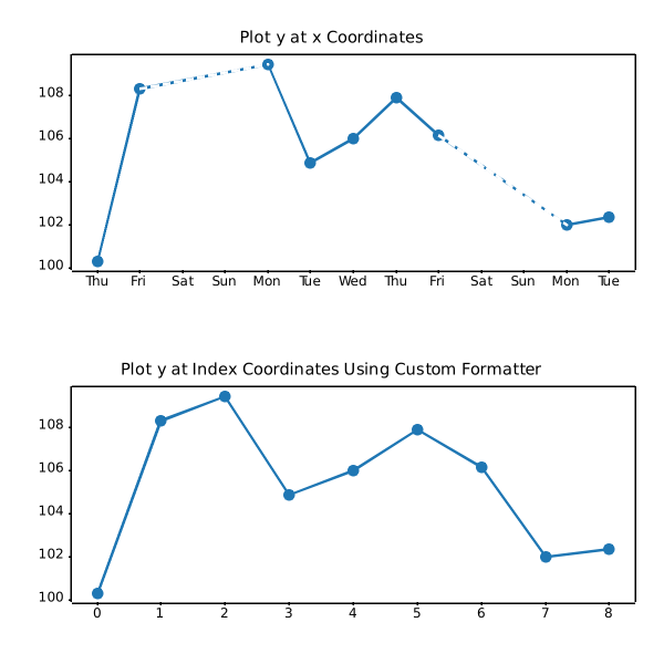
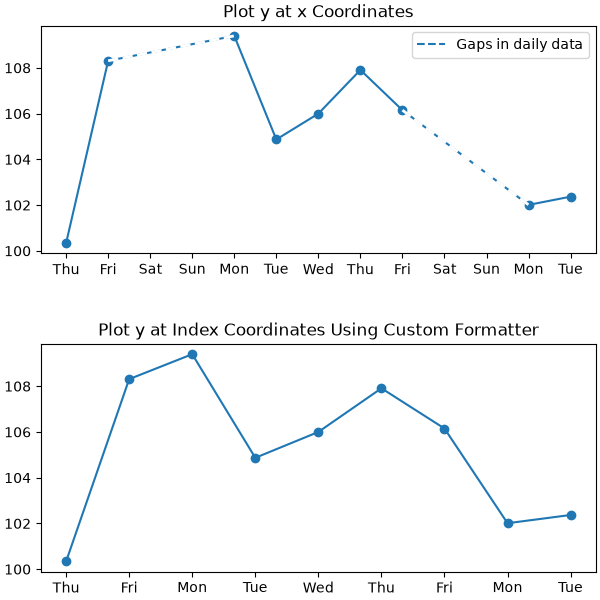
ticks/date_precision_and_epochs
=========================
Source
"""
=========================
Date precision and epochs
=========================
Matplotlib can handle `.datetime` objects and `numpy.datetime64` objects using
a unit converter that recognizes these dates and converts them to floating
point numbers.
Before Matplotlib 3.3, the default for this conversion returns a float that was
days since "0000-12-31T00:00:00". As of Matplotlib 3.3, the default is
days from "1970-01-01T00:00:00". This allows more resolution for modern
dates. "2020-01-01" with the old epoch converted to 730120, and a 64-bit
floating point number has a resolution of 2^{-52}, or approximately
14 microseconds, so microsecond precision was lost. With the new default
epoch "2020-01-01" is 10957.0, so the achievable resolution is 0.21
microseconds.
"""
import datetime
import matplotlib.pyplot as plt
import numpy as np
import matplotlib.dates as mdates
def _reset_epoch_for_tutorial():
"""
Users (and downstream libraries) should not use the private method of
resetting the epoch.
"""
mdates._reset_epoch_test_example()
# %%
# Datetime
# --------
#
# Python `.datetime` objects have microsecond resolution, so with the
# old default matplotlib dates could not round-trip full-resolution datetime
# objects.
old_epoch = '0000-12-31T00:00:00'
new_epoch = '1970-01-01T00:00:00'
_reset_epoch_for_tutorial() # Don't do this. Just for this tutorial.
mdates.set_epoch(old_epoch) # old epoch (pre MPL 3.3)
date1 = datetime.datetime(2000, 1, 1, 0, 10, 0, 12,
tzinfo=datetime.timezone.utc)
mdate1 = mdates.date2num(date1)
print('Before Roundtrip: ', date1, 'Matplotlib date:', mdate1)
date2 = mdates.num2date(mdate1)
print('After Roundtrip: ', date2)
# %%
# Note this is only a round-off error, and there is no problem for
# dates closer to the old epoch:
date1 = datetime.datetime(10, 1, 1, 0, 10, 0, 12,
tzinfo=datetime.timezone.utc)
mdate1 = mdates.date2num(date1)
print('Before Roundtrip: ', date1, 'Matplotlib date:', mdate1)
date2 = mdates.num2date(mdate1)
print('After Roundtrip: ', date2)
# %%
# If a user wants to use modern dates at microsecond precision, they
# can change the epoch using `.set_epoch`. However, the epoch has to be
# set before any date operations to prevent confusion between different
# epochs. Trying to change the epoch later will raise a `RuntimeError`.
try:
mdates.set_epoch(new_epoch) # this is the new MPL 3.3 default.
except RuntimeError as e:
print('RuntimeError:', str(e))
# %%
# For this tutorial, we reset the sentinel using a private method, but users
# should just set the epoch once, if at all.
_reset_epoch_for_tutorial() # Just being done for this tutorial.
mdates.set_epoch(new_epoch)
date1 = datetime.datetime(2020, 1, 1, 0, 10, 0, 12,
tzinfo=datetime.timezone.utc)
mdate1 = mdates.date2num(date1)
print('Before Roundtrip: ', date1, 'Matplotlib date:', mdate1)
date2 = mdates.num2date(mdate1)
print('After Roundtrip: ', date2)
# %%
# datetime64
# ----------
#
# `numpy.datetime64` objects have microsecond precision for a much larger
# timespace than `.datetime` objects. However, currently Matplotlib time is
# only converted back to datetime objects, which have microsecond resolution,
# and years that only span 0000 to 9999.
_reset_epoch_for_tutorial() # Don't do this. Just for this tutorial.
mdates.set_epoch(new_epoch)
date1 = np.datetime64('2000-01-01T00:10:00.000012')
mdate1 = mdates.date2num(date1)
print('Before Roundtrip: ', date1, 'Matplotlib date:', mdate1)
date2 = mdates.num2date(mdate1)
print('After Roundtrip: ', date2)
# %%
# Plotting
# --------
#
# This all of course has an effect on plotting. With the old default epoch
# the times were rounded during the internal ``date2num`` conversion, leading
# to jumps in the data:
_reset_epoch_for_tutorial() # Don't do this. Just for this tutorial.
mdates.set_epoch(old_epoch)
x = np.arange('2000-01-01T00:00:00.0', '2000-01-01T00:00:00.000100',
dtype='datetime64[us]')
# simulate the plot being made using the old epoch
xold = np.array([mdates.num2date(mdates.date2num(d)) for d in x])
y = np.arange(0, len(x))
# resetting the Epoch so plots are comparable
_reset_epoch_for_tutorial() # Don't do this. Just for this tutorial.
mdates.set_epoch(new_epoch)
fig, ax = plt.subplots(layout='constrained')
ax.plot(xold, y)
ax.set_title('Epoch: ' + mdates.get_epoch())
ax.xaxis.set_tick_params(rotation=40)
plt.show()
# %%
# For dates plotted using the more recent epoch, the plot is smooth:
fig, ax = plt.subplots(layout='constrained')
ax.plot(x, y)
ax.set_title('Epoch: ' + mdates.get_epoch())
ax.xaxis.set_tick_params(rotation=40)
plt.show()
_reset_epoch_for_tutorial() # Don't do this. Just for this tutorial.
# %%
#
# .. admonition:: References
#
# The use of the following functions, methods, classes and modules is shown
# in this example:
#
# - `matplotlib.dates.num2date`
# - `matplotlib.dates.date2num`
# - `matplotlib.dates.set_epoch`
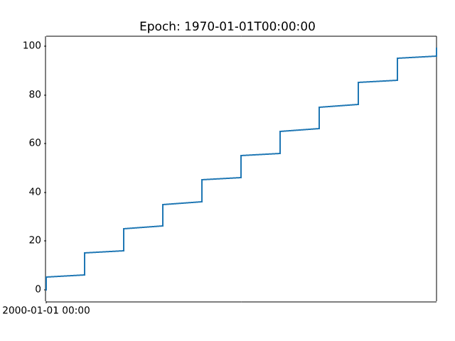
ticks/dollar_ticks
============
Source
"""
============
Dollar ticks
============
Use a format string to prepend dollar signs on y-axis labels.
.. redirect-from:: /gallery/pyplots/dollar_ticks
"""
import matplotlib.pyplot as plt
import numpy as np
# Fixing random state for reproducibility
np.random.seed(19680801)
fig, ax = plt.subplots()
ax.plot(100*np.random.rand(20))
# Use automatic StrMethodFormatter
ax.yaxis.set_major_formatter('${x:1.2f}')
ax.yaxis.set_tick_params(which='major', labelcolor='green',
labelleft=False, labelright=True)
plt.show()
# %%
#
# .. admonition:: References
#
# The use of the following functions, methods, classes and modules is shown
# in this example:
#
# - `matplotlib.pyplot.subplots`
# - `matplotlib.axis.Axis.set_major_formatter`
# - `matplotlib.axis.Axis.set_tick_params`
# - `matplotlib.axis.Tick`
# - `matplotlib.ticker.StrMethodFormatter`
ticks/engformatter_offset
===================================================
Source
"""
===================================================
SI prefixed offsets and natural order of magnitudes
===================================================
`matplotlib.ticker.EngFormatter` is capable of computing a natural
offset for your axis data, and presenting it with a standard SI prefix
automatically calculated.
Below is an examples of such a plot:
"""
import matplotlib.pyplot as plt
import numpy as np
import matplotlib.ticker as mticker
# Fixing random state for reproducibility
np.random.seed(19680801)
UNIT = "Hz"
fig, ax = plt.subplots()
ax.yaxis.set_major_formatter(mticker.EngFormatter(
useOffset=True,
unit=UNIT
))
size = 100
measurement = np.full(size, 1e9)
noise = np.random.uniform(low=-2e3, high=2e3, size=size)
ax.plot(measurement + noise)
plt.show()
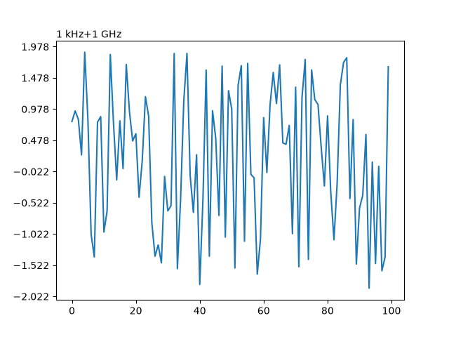
ticks/engineering_formatter
=======================================
Source
"""
=======================================
Format ticks using engineering notation
=======================================
Use of the engineering Formatter.
.. redirect-from:: /gallery/text_labels_and_annotations/engineering_formatter
"""
import matplotlib.pyplot as plt
import numpy as np
from matplotlib.ticker import EngFormatter
# Fixing random state for reproducibility
prng = np.random.RandomState(19680801)
# Create artificial data to plot.
# The x data span over several decades to demonstrate several SI prefixes.
xs = np.logspace(1, 9, 100)
ys = (0.8 + 0.4 * prng.uniform(size=100)) * np.log10(xs)**2
# Figure width is doubled (2*6.4) to display nicely 2 subplots side by side.
fig, (ax0, ax1) = plt.subplots(nrows=2, figsize=(7, 9.6))
for ax in (ax0, ax1):
ax.set_xscale('log')
# Demo of the default settings, with a user-defined unit label.
ax0.set_title('Full unit ticklabels, w/ default precision & space separator')
formatter0 = EngFormatter(unit='Hz')
ax0.xaxis.set_major_formatter(formatter0)
ax0.plot(xs, ys)
ax0.set_xlabel('Frequency')
# Demo of the options `places` (number of digit after decimal point) and
# `sep` (separator between the number and the prefix/unit).
ax1.set_title('SI-prefix only ticklabels, 1-digit precision & '
'thin space separator')
formatter1 = EngFormatter(places=1, sep="\N{THIN SPACE}") # U+2009
ax1.xaxis.set_major_formatter(formatter1)
ax1.plot(xs, ys)
ax1.set_xlabel('Frequency [Hz]')
plt.tight_layout()
plt.show()
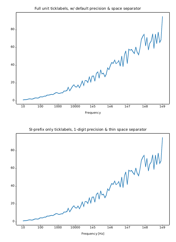
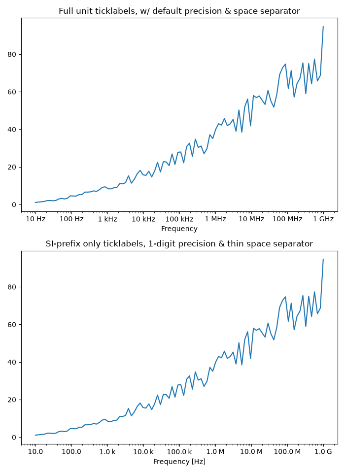
ticks/fig_axes_customize_simple
======================================
Source
"""
======================================
Customizing figure and axes appearance
======================================
Customize the background, labels and ticks of a simple plot.
.. redirect-from:: /gallery/pyplots/fig_axes_customize_simple
"""
import matplotlib.pyplot as plt
fig = plt.figure()
fig.patch.set_facecolor('lightgoldenrodyellow')
ax1 = fig.add_axes((0.1, 0.3, 0.4, 0.4))
ax1.patch.set_facecolor('lightslategray')
ax1.tick_params(axis='x', labelcolor='tab:red', labelrotation=45, labelsize=16)
ax1.tick_params(axis='y', color='tab:green', size=25, width=3)
plt.show()
# %%
#
# .. admonition:: References
#
# The use of the following functions, methods, classes and modules is shown
# in this example:
#
# - `matplotlib.axes.Axes.tick_params`
# - `matplotlib.patches.Patch.set_facecolor`
ticks/major_minor_demo
=====================
Source
r"""
=====================
Major and minor ticks
=====================
Demonstrate how to use major and minor tickers.
The two relevant classes are `.Locator`\s and `.Formatter`\s. Locators
determine where the ticks are, and formatters control the formatting of tick
labels.
Minor ticks are off by default (using `.NullLocator` and `.NullFormatter`).
Minor ticks can be turned on without labels by setting the minor locator.
Minor tick labels can be turned on by setting the minor formatter.
`.MultipleLocator` places ticks on multiples of some base.
`.StrMethodFormatter` uses a format string (e.g., ``'{x:d}'`` or ``'{x:1.2f}'``
or ``'{x:1.1f} cm'``) to format the tick labels (the variable in the format
string must be ``'x'``). For a `.StrMethodFormatter`, the string can be passed
directly to `.Axis.set_major_formatter` or
`.Axis.set_minor_formatter`. An appropriate `.StrMethodFormatter` will
be created and used automatically.
`.pyplot.grid` changes the grid settings of the major ticks of the x- and
y-axis together. If you want to control the grid of the minor ticks for a
given axis, use for example ::
ax.xaxis.grid(True, which='minor')
Note that a given locator or formatter instance can only be used on a single
axis (because the locator stores references to the axis data and view limits).
"""
import matplotlib.pyplot as plt
import numpy as np
from matplotlib.ticker import AutoMinorLocator, MultipleLocator
t = np.arange(0.0, 100.0, 0.1)
s = np.sin(0.1 * np.pi * t) * np.exp(-t * 0.01)
fig, ax = plt.subplots()
ax.plot(t, s)
# Make a plot with major ticks that are multiples of 20 and minor ticks that
# are multiples of 5. Label major ticks with '.0f' formatting but don't label
# minor ticks. The string is used directly, the `StrMethodFormatter` is
# created automatically.
ax.xaxis.set_major_locator(MultipleLocator(20))
ax.xaxis.set_major_formatter('{x:.0f}')
# For the minor ticks, use no labels; default NullFormatter.
ax.xaxis.set_minor_locator(MultipleLocator(5))
plt.show()
# %%
# Automatic tick selection for major and minor ticks.
#
# Use interactive pan and zoom to see how the tick intervals change. There will
# be either 4 or 5 minor tick intervals per major interval, depending on the
# major interval.
#
# One can supply an argument to `.AutoMinorLocator` to specify a fixed number
# of minor intervals per major interval, e.g. ``AutoMinorLocator(2)`` would
# lead to a single minor tick between major ticks.
t = np.arange(0.0, 100.0, 0.01)
s = np.sin(2 * np.pi * t) * np.exp(-t * 0.01)
fig, ax = plt.subplots()
ax.plot(t, s)
ax.xaxis.set_minor_locator(AutoMinorLocator())
ax.tick_params(which='both', width=2)
ax.tick_params(which='major', length=7)
ax.tick_params(which='minor', length=4, color='r')
plt.show()
# %%
#
# .. admonition:: References
#
# The use of the following functions, methods, classes and modules is shown
# in this example:
#
# - `matplotlib.pyplot.subplots`
# - `matplotlib.axis.Axis.set_major_formatter`
# - `matplotlib.axis.Axis.set_major_locator`
# - `matplotlib.axis.Axis.set_minor_locator`
# - `matplotlib.ticker.AutoMinorLocator`
# - `matplotlib.ticker.MultipleLocator`
# - `matplotlib.ticker.StrMethodFormatter`
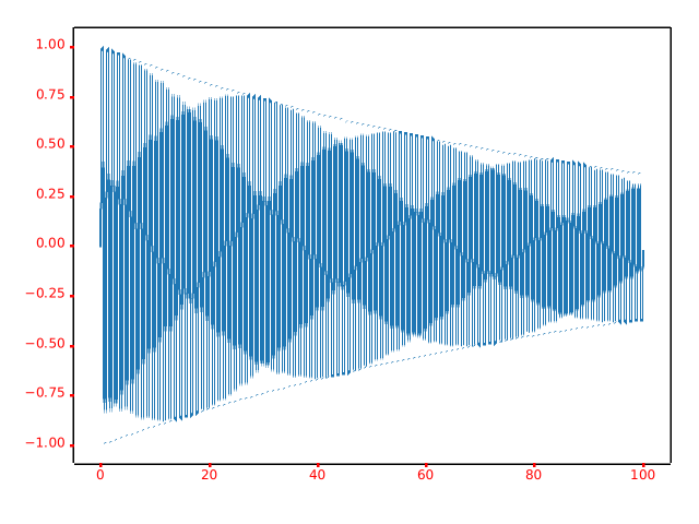
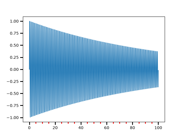
ticks/multilevel_ticks
=========================
Source
"""
=========================
Multilevel (nested) ticks
=========================
Sometimes we want another level of tick labels on an axis, perhaps to indicate
a grouping of the ticks.
Matplotlib does not provide an automated way to do this, but it is relatively
straightforward to annotate below the main axis.
These examples use `.Axes.secondary_xaxis`, which is one approach. It has the
advantage that we can use Matplotlib Locators and Formatters on the axis that
does the grouping if we want.
This first example creates a secondary xaxis and manually adds the ticks and
labels using `.Axes.set_xticks`. Note that the tick labels have a newline
(e.g. ``"\nOughts"``) at the beginning of them to put the second-level tick
labels below the main tick labels.
"""
import matplotlib.pyplot as plt
import numpy as np
import matplotlib.dates as mdates
rng = np.random.default_rng(19680801)
fig, ax = plt.subplots(layout='constrained', figsize=(4, 4))
ax.plot(np.arange(30))
sec = ax.secondary_xaxis(location=0)
sec.set_xticks([5, 15, 25], labels=['\nOughts', '\nTeens', '\nTwenties'])
# %%
# This second example adds a second level of annotation to a categorical axis.
# Here we need to note that each animal (category) is assigned an integer, so
# ``cats`` is at x=0, ``dogs`` at x=1 etc. Then we place the ticks on the
# second level on an x that is at the middle of the animal class we are trying
# to delineate.
#
# This example also adds tick marks between the classes by adding a second
# secondary xaxis, and placing long, wide ticks at the boundaries between the
# animal classes.
fig, ax = plt.subplots(layout='constrained', figsize=(7, 4))
ax.plot(['cats', 'dogs', 'pigs', 'snakes', 'lizards', 'chickens',
'eagles', 'herons', 'buzzards'],
rng.normal(size=9), 'o')
# label the classes:
sec = ax.secondary_xaxis(location=0)
sec.set_xticks([1, 3.5, 6.5], labels=['\n\nMammals', '\n\nReptiles', '\n\nBirds'])
sec.tick_params('x', length=0)
# lines between the classes:
sec2 = ax.secondary_xaxis(location=0)
sec2.set_xticks([-0.5, 2.5, 4.5, 8.5], labels=[])
sec2.tick_params('x', length=40, width=1.5)
ax.set_xlim(-0.6, 8.6)
# %%
# Dates are another common place where we may want to have a second level of
# tick labels. In this last example, we take advantage of the ability to add
# an automatic locator and formatter to the secondary xaxis, which means we do
# not need to set the ticks manually.
#
# This example also differs from the above, in that we placed it at a location
# below the main axes ``location=-0.075`` and then we hide the spine by setting
# the line width to zero. That means that our formatter no longer needs the
# carriage returns of the previous two examples.
fig, ax = plt.subplots(layout='constrained', figsize=(7, 4))
time = np.arange(np.datetime64('2020-01-01'), np.datetime64('2020-03-31'),
np.timedelta64(1, 'D'))
ax.plot(time, rng.random(size=len(time)))
# just format the days:
ax.xaxis.set_major_formatter(mdates.DateFormatter('%d'))
# label the months:
sec = ax.secondary_xaxis(location=-0.075)
sec.xaxis.set_major_locator(mdates.MonthLocator(bymonthday=1))
# note the extra spaces in the label to align the month label inside the month.
# Note that this could have been done by changing ``bymonthday`` above as well:
sec.xaxis.set_major_formatter(mdates.DateFormatter(' %b'))
sec.tick_params('x', length=0)
sec.spines['bottom'].set_linewidth(0)
# label the xaxis, but note for this to look good, it needs to be on the
# secondary xaxis.
sec.set_xlabel('Dates (2020)')
plt.show()
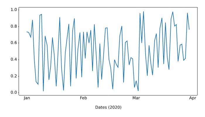
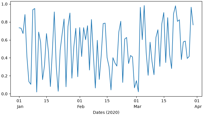
ticks/scalarformatter
==========================
Source
"""
==========================
The default tick formatter
==========================
By default, tick labels are formatted using a `.ScalarFormatter`, which can be
configured via `~.axes.Axes.ticklabel_format`. This example illustrates some
possible configurations:
- Default.
- ``useMathText=True``: Fancy formatting of mathematical expressions.
- ``useOffset=False``: Do not use offset notation; see
`.ScalarFormatter.set_useOffset`.
"""
import matplotlib.pyplot as plt
import numpy as np
x = np.arange(0, 1, .01)
fig, axs = plt.subplots(
3, 3, figsize=(9, 9), layout="constrained", gridspec_kw={"hspace": 0.1})
for col in axs.T:
col[0].plot(x * 1e5 + 1e10, x * 1e-10 + 1e-5)
col[1].plot(x * 1e5, x * 1e-4)
col[2].plot(-x * 1e5 - 1e10, -x * 1e-5 - 1e-10)
for ax in axs[:, 1]:
ax.ticklabel_format(useMathText=True)
for ax in axs[:, 2]:
ax.ticklabel_format(useOffset=False)
plt.rcParams.update({"axes.titleweight": "bold", "axes.titley": 1.1})
axs[0, 0].set_title("default settings")
axs[0, 1].set_title("useMathText=True")
axs[0, 2].set_title("useOffset=False")
plt.show()
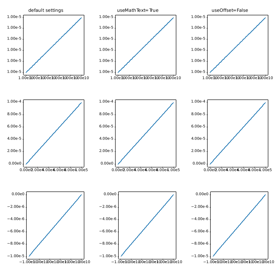
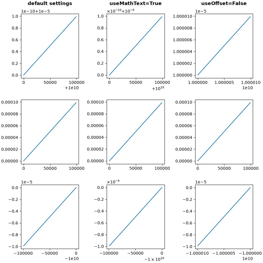
ticks/tick-formatters
===============
Source
"""
===============
Tick formatters
===============
Tick formatters define how the numeric value associated with a tick on an axis
is formatted as a string.
This example illustrates the usage and effect of the most common formatters.
The tick format is configured via the function `~.Axis.set_major_formatter`
or `~.Axis.set_minor_formatter`. It accepts:
- a format string, which implicitly creates a `.StrMethodFormatter`.
- a function, implicitly creates a `.FuncFormatter`.
- an instance of a `.Formatter` subclass. The most common are
- `.NullFormatter`: No labels on the ticks.
- `.StrMethodFormatter`: Use string `str.format` method.
- `.FormatStrFormatter`: Use %-style formatting.
- `.FuncFormatter`: Define labels through a function.
- `.FixedFormatter`: Set the label strings explicitly.
- `.ScalarFormatter`: Default formatter for scalars: auto-pick the format string.
- `.PercentFormatter`: Format labels as a percentage.
See :ref:`formatters` for a complete list.
"""
import matplotlib.pyplot as plt
from matplotlib import ticker
def setup(ax, title):
"""Set up common parameters for the Axes in the example."""
# only show the bottom spine
ax.yaxis.set_major_locator(ticker.NullLocator())
ax.spines[['left', 'right', 'top']].set_visible(False)
# define tick positions
ax.xaxis.set_major_locator(ticker.MultipleLocator(1.00))
ax.xaxis.set_minor_locator(ticker.MultipleLocator(0.25))
ax.xaxis.set_ticks_position('bottom')
ax.tick_params(which='major', width=1.00, length=5)
ax.tick_params(which='minor', width=0.75, length=2.5, labelsize=10)
ax.set_xlim(0, 5)
ax.set_ylim(0, 1)
ax.text(0.0, 0.2, title, transform=ax.transAxes,
fontsize=14, fontname='Monospace', color='tab:blue')
fig = plt.figure(figsize=(8, 8), layout='constrained')
fig0, fig1, fig2 = fig.subfigures(3, height_ratios=[1.5, 1.5, 7.5])
fig0.suptitle('String Formatting', fontsize=16, x=0, ha='left')
ax0 = fig0.subplots()
setup(ax0, title="'{x} km'")
ax0.xaxis.set_major_formatter('{x} km')
fig1.suptitle('Function Formatting', fontsize=16, x=0, ha='left')
ax1 = fig1.subplots()
setup(ax1, title="def(x, pos): return str(x-5)")
ax1.xaxis.set_major_formatter(lambda x, pos: str(x-5))
fig2.suptitle('Formatter Object Formatting', fontsize=16, x=0, ha='left')
axs2 = fig2.subplots(7, 1)
setup(axs2[0], title="NullFormatter()")
axs2[0].xaxis.set_major_formatter(ticker.NullFormatter())
setup(axs2[1], title="StrMethodFormatter('{x:.3f}')")
axs2[1].xaxis.set_major_formatter(ticker.StrMethodFormatter("{x:.3f}"))
setup(axs2[2], title="FormatStrFormatter('#%d')")
axs2[2].xaxis.set_major_formatter(ticker.FormatStrFormatter("#%d"))
def fmt_two_digits(x, pos):
return f'[{x:.2f}]'
setup(axs2[3], title='FuncFormatter("[{:.2f}]".format)')
axs2[3].xaxis.set_major_formatter(ticker.FuncFormatter(fmt_two_digits))
setup(axs2[4], title="FixedFormatter(['A', 'B', 'C', 'D', 'E', 'F'])")
# FixedFormatter should only be used together with FixedLocator.
# Otherwise, one cannot be sure where the labels will end up.
positions = [0, 1, 2, 3, 4, 5]
labels = ['A', 'B', 'C', 'D', 'E', 'F']
axs2[4].xaxis.set_major_locator(ticker.FixedLocator(positions))
axs2[4].xaxis.set_major_formatter(ticker.FixedFormatter(labels))
setup(axs2[5], title="ScalarFormatter()")
axs2[5].xaxis.set_major_formatter(ticker.ScalarFormatter(useMathText=True))
setup(axs2[6], title="PercentFormatter(xmax=5)")
axs2[6].xaxis.set_major_formatter(ticker.PercentFormatter(xmax=5))
plt.show()
# %%
# .. tags:: component: ticks, purpose: reference
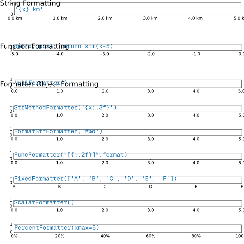
ticks/tick-locators
=============
Source
"""
=============
Tick locators
=============
Tick locators define the position of the ticks.
This example illustrates the usage and effect of the most common locators.
"""
import matplotlib.pyplot as plt
import numpy as np
import matplotlib.ticker as ticker
def setup(ax, title):
"""Set up common parameters for the Axes in the example."""
# only show the bottom spine
ax.yaxis.set_major_locator(ticker.NullLocator())
ax.spines[['left', 'right', 'top']].set_visible(False)
ax.xaxis.set_ticks_position('bottom')
ax.tick_params(which='major', width=1.00, length=5)
ax.tick_params(which='minor', width=0.75, length=2.5)
ax.set_xlim(0, 5)
ax.set_ylim(0, 1)
ax.text(0.0, 0.2, title, transform=ax.transAxes,
fontsize=14, fontname='Monospace', color='tab:blue')
fig, axs = plt.subplots(8, 1, figsize=(8, 6))
# Null Locator
setup(axs[0], title="NullLocator()")
axs[0].xaxis.set_major_locator(ticker.NullLocator())
axs[0].xaxis.set_minor_locator(ticker.NullLocator())
# Multiple Locator
setup(axs[1], title="MultipleLocator(0.5, offset=0.2)")
axs[1].xaxis.set_major_locator(ticker.MultipleLocator(0.5, offset=0.2))
axs[1].xaxis.set_minor_locator(ticker.MultipleLocator(0.1))
# Fixed Locator
setup(axs[2], title="FixedLocator([0, 1, 5])")
axs[2].xaxis.set_major_locator(ticker.FixedLocator([0, 1, 5]))
axs[2].xaxis.set_minor_locator(ticker.FixedLocator(np.linspace(0.2, 0.8, 4)))
# Linear Locator
setup(axs[3], title="LinearLocator(numticks=3)")
axs[3].xaxis.set_major_locator(ticker.LinearLocator(3))
axs[3].xaxis.set_minor_locator(ticker.LinearLocator(31))
# Index Locator
setup(axs[4], title="IndexLocator(base=0.5, offset=0.25)")
axs[4].plot([0]*5, color='white')
axs[4].xaxis.set_major_locator(ticker.IndexLocator(base=0.5, offset=0.25))
# Auto Locator
setup(axs[5], title="AutoLocator()")
axs[5].xaxis.set_major_locator(ticker.AutoLocator())
axs[5].xaxis.set_minor_locator(ticker.AutoMinorLocator())
# MaxN Locator
setup(axs[6], title="MaxNLocator(n=4)")
axs[6].xaxis.set_major_locator(ticker.MaxNLocator(4))
axs[6].xaxis.set_minor_locator(ticker.MaxNLocator(40))
# Log Locator
setup(axs[7], title="LogLocator(base=10, numticks=15)")
axs[7].set_xlim(10**3, 10**10)
axs[7].set_xscale('log')
axs[7].xaxis.set_major_locator(ticker.LogLocator(base=10, numticks=15))
plt.tight_layout()
plt.show()
# %%
#
# .. admonition:: References
#
# The following functions, methods, classes and modules are used in this example:
#
# - `matplotlib.axis.Axis.set_major_locator`
# - `matplotlib.axis.Axis.set_minor_locator`
# - `matplotlib.ticker.NullLocator`
# - `matplotlib.ticker.MultipleLocator`
# - `matplotlib.ticker.FixedLocator`
# - `matplotlib.ticker.LinearLocator`
# - `matplotlib.ticker.IndexLocator`
# - `matplotlib.ticker.AutoLocator`
# - `matplotlib.ticker.MaxNLocator`
# - `matplotlib.ticker.LogLocator`
#
# .. tags:: component: ticks, purpose: reference
ticks/tick_labels_from_values
=========================================
Source
"""
=========================================
Setting tick labels from a list of values
=========================================
Using `.Axes.set_xticks` causes the tick labels to be set on the currently
chosen ticks. However, you may want to allow matplotlib to dynamically
choose the number of ticks and their spacing.
In this case it may be better to determine the tick label from the
value at the tick. The following example shows how to do this.
NB: The `.ticker.MaxNLocator` is used here to ensure that the tick values
take integer values.
"""
import matplotlib.pyplot as plt
from matplotlib.ticker import MaxNLocator
fig, ax = plt.subplots()
xs = range(26)
ys = range(26)
labels = list('abcdefghijklmnopqrstuvwxyz')
def format_fn(tick_val, tick_pos):
if int(tick_val) in xs:
return labels[int(tick_val)]
else:
return ''
# A FuncFormatter is created automatically.
ax.xaxis.set_major_formatter(format_fn)
ax.xaxis.set_major_locator(MaxNLocator(integer=True))
ax.plot(xs, ys)
plt.show()
# %%
#
# .. admonition:: References
#
# The use of the following functions, methods, classes and modules is shown
# in this example:
#
# - `matplotlib.pyplot.subplots`
# - `matplotlib.axis.Axis.set_major_formatter`
# - `matplotlib.axis.Axis.set_major_locator`
# - `matplotlib.ticker.FuncFormatter`
# - `matplotlib.ticker.MaxNLocator`
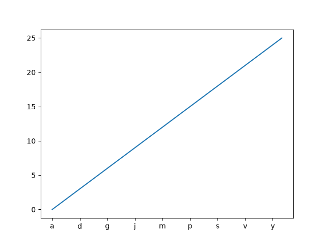
ticks/ticklabels_rotation
===================
Source
"""
===================
Rotated tick labels
===================
Rotating tick labels can be useful when the labels are long and overlap with each other.
Adjust the tick properties using `~.Axes.tick_params`: Set the angle in degrees via
the *rotation* parameter. Set the *rotation_mode* parameter to "xtick" / "ytick" to
make the text point towards the tick, see also `~.Text.set_rotation_mode`.
Note: We use ``layout="constrained"`` to make sure there is enough space for the tick
labels so that they are not cut off.
"""
import matplotlib.pyplot as plt
population = {
'India': 1417.492,
'China': 1404.89,
'United States': 341.784857,
'Indonesia': 284.438782,
'Pakistan': 241.499431,
'Nigeria': 223.8,
'Brazil': 213.421037,
'Bangladesh': 169.828911,
'Russia': 146.028325,
'Mexico': 131.001723,
'Japan': 122.95,
'Philippines': 114.1236,
'DR Congo': 112.832,
'Ethiopia': 111.652998,
'Egypt': 107.868296,
'Vietnam': 102.3,
}
fig, ax = plt.subplots(layout="constrained")
ax.bar(population.keys(), population.values())
ax.tick_params("x", rotation=45, rotation_mode="xtick")
ax.set_ylabel("population (millions)")
plt.show()
# %%
#
# .. admonition:: References
#
# The use of the following functions, methods, classes and modules is shown
# in this example:
#
# - `matplotlib.axes.Axes.tick_params` / `matplotlib.pyplot.tick_params`
#
# .. tags:: component: ticks, plot-type: bar
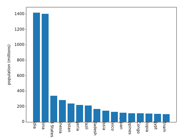
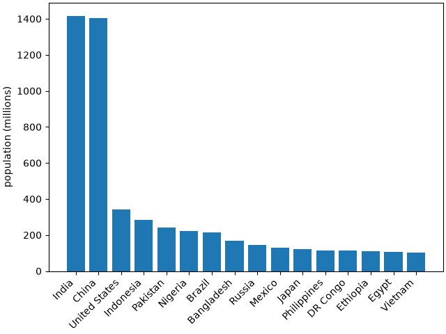
ticks/ticks_too_many
=====================
Source
"""
=====================
Fixing too many ticks
=====================
One common cause for unexpected tick behavior is passing a list of strings
instead of numbers or datetime objects. This can easily happen without notice
when reading in a comma-delimited text file. Matplotlib treats lists of strings
as *categorical* variables
(:doc:`/gallery/lines_bars_and_markers/categorical_variables`), and by default
puts one tick per category, and plots them in the order in which they are
supplied. If this is not desired, the solution is to convert the strings to
a numeric type as in the following examples.
"""
# %%
# Example 1: Strings can lead to an unexpected order of number ticks
# ------------------------------------------------------------------
import matplotlib.pyplot as plt
import numpy as np
fig, ax = plt.subplots(1, 2, layout='constrained', figsize=(6, 2.5))
x = ['1', '5', '2', '3']
y = [1, 4, 2, 3]
ax[0].plot(x, y, 'd')
ax[0].tick_params(axis='x', color='r', labelcolor='r')
ax[0].set_xlabel('Categories')
ax[0].set_title('Ticks seem out of order / misplaced')
# convert to numbers:
x = np.asarray(x, dtype='float')
ax[1].plot(x, y, 'd')
ax[1].set_xlabel('Floats')
ax[1].set_title('Ticks as expected')
# %%
# Example 2: Strings can lead to very many ticks
# ----------------------------------------------
# If *x* has 100 elements, all strings, then we would have 100 (unreadable)
# ticks, and again the solution is to convert the strings to floats:
fig, ax = plt.subplots(1, 2, figsize=(6, 2.5))
x = [f'{xx}' for xx in np.arange(100)]
y = np.arange(100)
ax[0].plot(x, y)
ax[0].tick_params(axis='x', color='r', labelcolor='r')
ax[0].set_title('Too many ticks')
ax[0].set_xlabel('Categories')
ax[1].plot(np.asarray(x, float), y)
ax[1].set_title('x converted to numbers')
ax[1].set_xlabel('Floats')
# %%
# Example 3: Strings can lead to an unexpected order of datetime ticks
# --------------------------------------------------------------------
# A common case is when dates are read from a CSV file, they need to be
# converted from strings to datetime objects to get the proper date locators
# and formatters.
fig, ax = plt.subplots(1, 2, layout='constrained', figsize=(6, 2.75))
x = ['2021-10-01', '2021-11-02', '2021-12-03', '2021-09-01']
y = [0, 2, 3, 1]
ax[0].plot(x, y, 'd')
ax[0].tick_params(axis='x', labelrotation=90, color='r', labelcolor='r')
ax[0].set_title('Dates out of order')
# convert to datetime64
x = np.asarray(x, dtype='datetime64[s]')
ax[1].plot(x, y, 'd')
ax[1].tick_params(axis='x', labelrotation=90)
ax[1].set_title('x converted to datetimes')
plt.show()
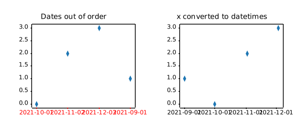
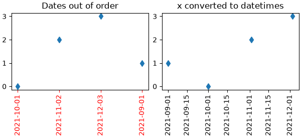
ticks/ticks_top_right
===============================================
Source
"""
===============================================
Move x/y-axis ticks and labels on top and right
===============================================
`.axes.Axes.tick_params` can be used to move tick marks and tick labels
to the top or right side of the Axes::
ax.tick_params(top=True, labeltop=True, bottom=False, labelbottom=False)
ax.tick_params(right=True, labelright=True, left=False, labelleft=False)
To also reposition the axes labels (xlabel/ylabel), use
``Axes.xaxis.set_label_position`` and ``Axes.yaxis.set_label_position``.
.. note::
To apply this globally for all future plots, set the rcParams:
- :rc:`xtick.top`
- :rc:`xtick.labeltop`
- :rc:`xtick.bottom`
- :rc:`xtick.labelbottom`
- :rc:`ytick.right`
- :rc:`ytick.labelright`
- :rc:`ytick.left`
- :rc:`ytick.labelleft`
.. redirect-from:: /gallery/ticks/tick_xlabel_top
.. redirect-from:: /gallery/ticks/tick_label_right
"""
import matplotlib.pyplot as plt
fig, ax = plt.subplots()
ax.plot(range(10))
# Move ticks marks and tick labels
ax.tick_params(
top=True, labeltop=True,
bottom=False, labelbottom=False,
right=True, labelright=True,
left=False, labelleft=False,
)
# Move axis labels
ax.xaxis.set_label_position("top")
ax.yaxis.set_label_position("right")
ax.set_xlabel("X label")
ax.set_ylabel("Y label")
plt.show()
units/annotate_with_units
=====================
Source
"""
=====================
Annotation with units
=====================
The example illustrates how to create text and arrow
annotations using a centimeter-scale plot.
.. only:: builder_html
This example requires :download:`basic_units.py <basic_units.py>`
"""
from basic_units import cm
import matplotlib.pyplot as plt
fig, ax = plt.subplots()
ax.annotate("Note 01", [0.5*cm, 0.5*cm])
# xy and text both unitized
ax.annotate('local max', xy=(3*cm, 1*cm), xycoords='data',
xytext=(0.8*cm, 0.95*cm), textcoords='data',
arrowprops=dict(facecolor='black', shrink=0.05),
horizontalalignment='right', verticalalignment='top')
# mixing units w/ nonunits
ax.annotate('local max', xy=(3*cm, 1*cm), xycoords='data',
xytext=(0.8, 0.95), textcoords='axes fraction',
arrowprops=dict(facecolor='black', shrink=0.05),
horizontalalignment='right', verticalalignment='top')
ax.set_xlim(0*cm, 4*cm)
ax.set_ylim(0*cm, 4*cm)
plt.show()
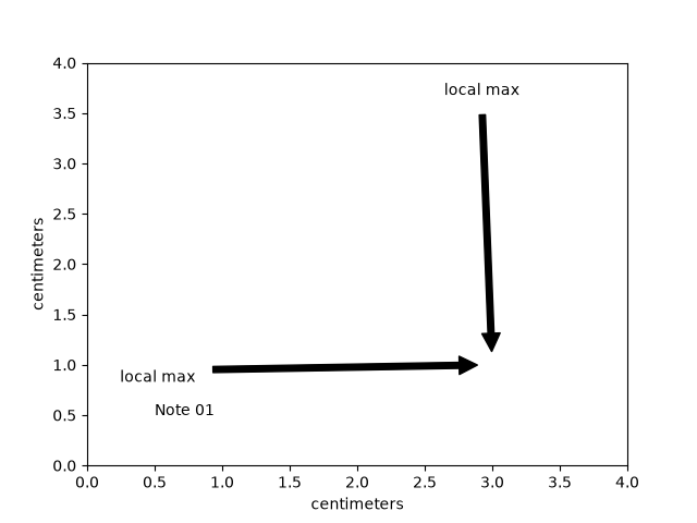
units/artist_tests
============
Source
"""
============
Artist tests
============
Test unit support with each of the Matplotlib primitive artist types.
The axis handles unit conversions and the artists keep a pointer to their axis
parent. You must initialize the artists with the axis instance if you want to
use them with unit data, or else they will not know how to convert the units
to scalars.
.. only:: builder_html
This example requires :download:`basic_units.py <basic_units.py>`
"""
import random
from basic_units import cm, inch
import matplotlib.pyplot as plt
import numpy as np
import matplotlib.collections as collections
import matplotlib.lines as lines
import matplotlib.patches as patches
import matplotlib.text as text
fig, ax = plt.subplots()
ax.xaxis.set_units(cm)
ax.yaxis.set_units(cm)
# Fixing random state for reproducibility
np.random.seed(19680801)
if 0:
# test a line collection
# Not supported at present.
verts = []
for i in range(10):
# a random line segment in inches
verts.append(zip(*inch*10*np.random.rand(2, random.randint(2, 15))))
lc = collections.LineCollection(verts, axes=ax)
ax.add_collection(lc)
# test a plain-ol-line
line = lines.Line2D([0*cm, 1.5*cm], [0*cm, 2.5*cm],
lw=2, color='black', axes=ax)
ax.add_line(line)
if 0:
# test a patch
# Not supported at present.
rect = patches.Rectangle((1*cm, 1*cm), width=5*cm, height=2*cm,
alpha=0.2, axes=ax)
ax.add_patch(rect)
t = text.Text(3*cm, 2.5*cm, 'text label', ha='left', va='bottom', axes=ax)
ax.add_artist(t)
ax.set_xlim(-1*cm, 10*cm)
ax.set_ylim(-1*cm, 10*cm)
# ax.xaxis.set_units(inch)
ax.grid(True)
ax.set_title("Artists with units")
plt.show()
units/bar_demo2
===================
Source
""" =================== Bar demo with units =================== A plot using a variety of centimetre and inch conversions. This example shows how default unit introspection works (ax1), how various keywords can be used to set the x and y units to override the defaults (ax2, ax3, ax4) and how one can set the xlimits using scalars (ax3, current units assumed) or units (conversions applied to get the numbers to current units). .. only:: builder_html This example requires :download:`basic_units.py <basic_units.py>` """ from basic_units import cm, inch import matplotlib.pyplot as plt import numpy as np cms = cm * np.arange(0, 10, 2) bottom = 0 * cm width = 0.8 * cm fig, axs = plt.subplots(2, 2) axs[0, 0].bar(cms, cms, bottom=bottom) axs[0, 1].bar(cms, cms, bottom=bottom, width=width, xunits=cm, yunits=inch) axs[1, 0].bar(cms, cms, bottom=bottom, width=width, xunits=inch, yunits=cm) axs[1, 0].set_xlim(2, 6) # scalars are interpreted in current units axs[1, 1].bar(cms, cms, bottom=bottom, width=width, xunits=inch, yunits=inch) axs[1, 1].set_xlim(2 * cm, 6 * cm) # cm are converted to inches fig.tight_layout() plt.show()
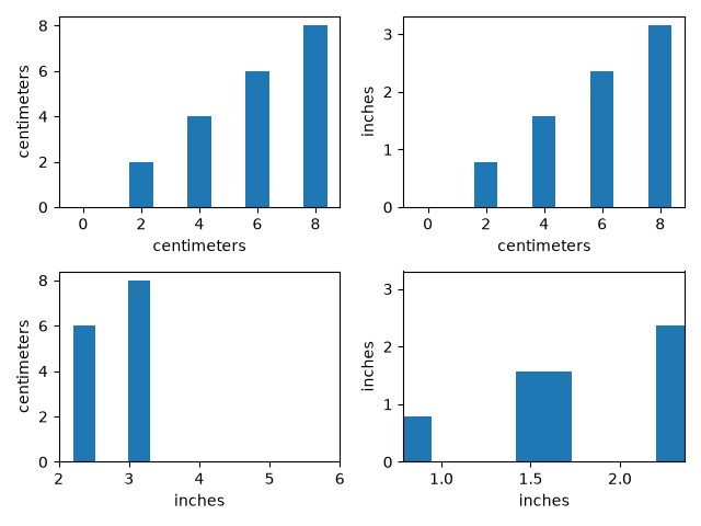
units/bar_unit_demo
=========================
Source
"""
=========================
Group barchart with units
=========================
This is the same example as
:doc:`the barchart</gallery/lines_bars_and_markers/barchart>` in
centimeters.
.. only:: builder_html
This example requires :download:`basic_units.py <basic_units.py>`
"""
from basic_units import cm, inch
import matplotlib.pyplot as plt
import numpy as np
N = 5
tea_means = [15*cm, 10*cm, 8*cm, 12*cm, 5*cm]
tea_std = [2*cm, 1*cm, 1*cm, 4*cm, 2*cm]
fig, ax = plt.subplots()
ax.yaxis.set_units(inch)
ind = np.arange(N) # the x locations for the groups
width = 0.35 # the width of the bars
ax.bar(ind, tea_means, width, bottom=0*cm, yerr=tea_std, label='Tea')
coffee_means = (14*cm, 19*cm, 7*cm, 5*cm, 10*cm)
coffee_std = (3*cm, 5*cm, 2*cm, 1*cm, 2*cm)
ax.bar(ind + width, coffee_means, width, bottom=0*cm, yerr=coffee_std,
label='Coffee')
ax.set_title('Cup height by group and beverage choice')
ax.set_xticks(ind + width / 2, labels=['G1', 'G2', 'G3', 'G4', 'G5'])
ax.legend()
ax.autoscale_view()
plt.show()
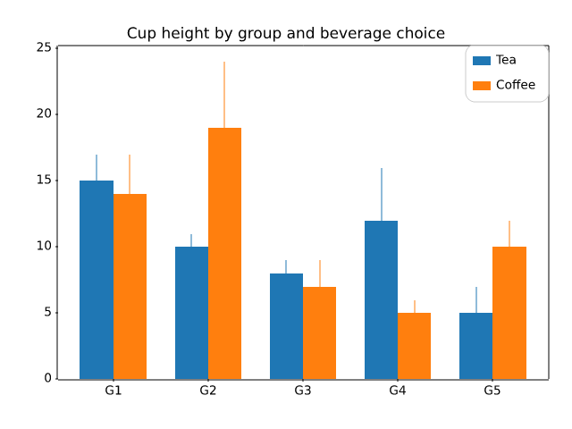
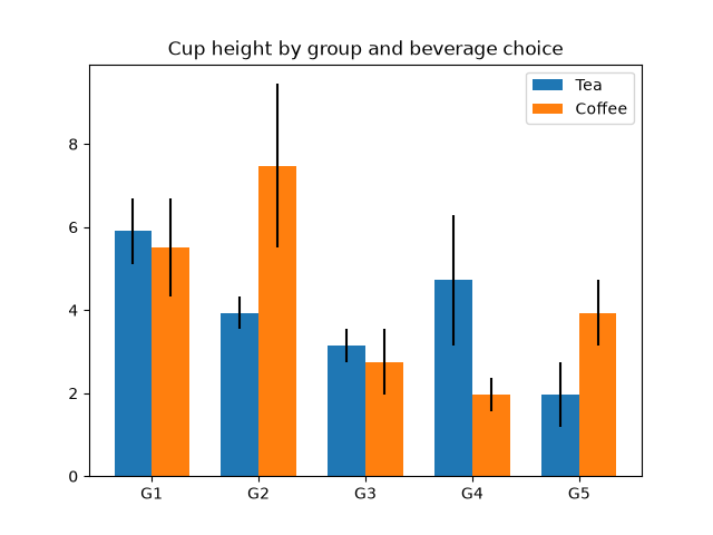
units/basic_units
.. _basic_units:
Source
"""
.. _basic_units:
===========
Basic units
===========
This file implements a units library that supports registering arbitrary units,
conversions between units, and math with unitized data. This library also implements a
Matplotlib unit converter and registers its units with Matplotlib. This library is used
in the examples to demonstrate Matplotlib's unit support. It is only maintained for the
purposes of building documentation and should never be used outside of the Matplotlib
documentation.
"""
import itertools
import math
from packaging.version import parse as parse_version
import numpy as np
import matplotlib.ticker as ticker
import matplotlib.units as units
class ProxyDelegate:
def __init__(self, fn_name, proxy_type):
self.proxy_type = proxy_type
self.fn_name = fn_name
def __get__(self, obj, objtype=None):
return self.proxy_type(self.fn_name, obj)
class TaggedValueMeta(type):
def __init__(self, name, bases, dict):
for fn_name in self._proxies:
if not hasattr(self, fn_name):
setattr(self, fn_name,
ProxyDelegate(fn_name, self._proxies[fn_name]))
class PassThroughProxy:
def __init__(self, fn_name, obj):
self.fn_name = fn_name
self.target = obj.proxy_target
def __call__(self, *args):
fn = getattr(self.target, self.fn_name)
ret = fn(*args)
return ret
class ConvertArgsProxy(PassThroughProxy):
def __init__(self, fn_name, obj):
super().__init__(fn_name, obj)
self.unit = obj.unit
def __call__(self, *args):
converted_args = []
for a in args:
try:
converted_args.append(a.convert_to(self.unit))
except AttributeError:
converted_args.append(TaggedValue(a, self.unit))
converted_args = tuple([c.get_value() for c in converted_args])
return super().__call__(*converted_args)
class ConvertReturnProxy(PassThroughProxy):
def __init__(self, fn_name, obj):
super().__init__(fn_name, obj)
self.unit = obj.unit
def __call__(self, *args):
ret = super().__call__(*args)
return (NotImplemented if ret is NotImplemented
else TaggedValue(ret, self.unit))
class ConvertAllProxy(PassThroughProxy):
def __init__(self, fn_name, obj):
super().__init__(fn_name, obj)
self.unit = obj.unit
def __call__(self, *args):
converted_args = []
arg_units = [self.unit]
for a in args:
if hasattr(a, 'get_unit') and not hasattr(a, 'convert_to'):
# If this argument has a unit type but no conversion ability,
# this operation is prohibited.
return NotImplemented
if hasattr(a, 'convert_to'):
try:
a = a.convert_to(self.unit)
except Exception:
pass
arg_units.append(a.get_unit())
converted_args.append(a.get_value())
else:
converted_args.append(a)
if hasattr(a, 'get_unit'):
arg_units.append(a.get_unit())
else:
arg_units.append(None)
converted_args = tuple(converted_args)
ret = super().__call__(*converted_args)
if ret is NotImplemented:
return NotImplemented
ret_unit = unit_resolver(self.fn_name, arg_units)
if ret_unit is NotImplemented:
return NotImplemented
return TaggedValue(ret, ret_unit)
class TaggedValue(metaclass=TaggedValueMeta):
_proxies = {'__add__': ConvertAllProxy,
'__sub__': ConvertAllProxy,
'__mul__': ConvertAllProxy,
'__rmul__': ConvertAllProxy,
'__cmp__': ConvertAllProxy,
'__lt__': ConvertAllProxy,
'__gt__': ConvertAllProxy,
'__len__': PassThroughProxy}
def __new__(cls, value, unit):
# generate a new subclass for value
value_class = type(value)
try:
subcls = type(f'TaggedValue_of_{value_class.__name__}',
(cls, value_class), {})
return object.__new__(subcls)
except TypeError:
return object.__new__(cls)
def __init__(self, value, unit):
self.value = value
self.unit = unit
self.proxy_target = self.value
def __copy__(self):
return TaggedValue(self.value, self.unit)
def __getattribute__(self, name):
if name.startswith('__'):
return object.__getattribute__(self, name)
variable = object.__getattribute__(self, 'value')
if hasattr(variable, name) and name not in self.__class__.__dict__:
return getattr(variable, name)
return object.__getattribute__(self, name)
def __array__(self, dtype=object, copy=False):
return np.asarray(self.value, dtype)
def __array_wrap__(self, array, context=None, return_scalar=False):
return TaggedValue(array, self.unit)
def __repr__(self):
return f'TaggedValue({self.value!r}, {self.unit!r})'
def __str__(self):
return f"{self.value} in {self.unit}"
def __len__(self):
return len(self.value)
if parse_version(np.__version__) >= parse_version('1.20'):
def __getitem__(self, key):
return TaggedValue(self.value[key], self.unit)
def __iter__(self):
# Return a generator expression rather than use `yield`, so that
# TypeError is raised by iter(self) if appropriate when checking for
# iterability.
return (TaggedValue(inner, self.unit) for inner in self.value)
def get_compressed_copy(self, mask):
new_value = np.ma.masked_array(self.value, mask=mask).compressed()
return TaggedValue(new_value, self.unit)
def convert_to(self, unit):
if unit == self.unit or not unit:
return self
try:
new_value = self.unit.convert_value_to(self.value, unit)
except AttributeError:
new_value = self
return TaggedValue(new_value, unit)
def get_value(self):
return self.value
def get_unit(self):
return self.unit
class BasicUnit:
# numpy scalars convert eager and np.float64(2) * BasicUnit('cm')
# would thus return a numpy scalar. To avoid this, we increase the
# priority of the BasicUnit.
__array_priority__ = np.float64(0).__array_priority__ + 1
def __init__(self, name, fullname=None):
self.name = name
if fullname is None:
fullname = name
self.fullname = fullname
self.conversions = dict()
def __repr__(self):
return f'BasicUnit({self.name})'
def __str__(self):
return self.fullname
def __call__(self, value):
return TaggedValue(value, self)
def __mul__(self, rhs):
value = rhs
unit = self
if hasattr(rhs, 'get_unit'):
value = rhs.get_value()
unit = rhs.get_unit()
unit = unit_resolver('__mul__', (self, unit))
if unit is NotImplemented:
return NotImplemented
return TaggedValue(value, unit)
def __rmul__(self, lhs):
return self*lhs
def __array_wrap__(self, array, context=None, return_scalar=False):
return TaggedValue(array, self)
def __array__(self, t=None, context=None, copy=False):
ret = np.array(1)
if t is not None:
return ret.astype(t)
else:
return ret
def add_conversion_factor(self, unit, factor):
def convert(x):
return x*factor
self.conversions[unit] = convert
def add_conversion_fn(self, unit, fn):
self.conversions[unit] = fn
def get_conversion_fn(self, unit):
return self.conversions[unit]
def convert_value_to(self, value, unit):
conversion_fn = self.conversions[unit]
ret = conversion_fn(value)
return ret
def get_unit(self):
return self
class UnitResolver:
def addition_rule(self, units):
for unit_1, unit_2 in itertools.pairwise(units):
if unit_1 != unit_2:
return NotImplemented
return units[0]
def multiplication_rule(self, units):
non_null = [u for u in units if u]
if len(non_null) > 1:
return NotImplemented
return non_null[0]
op_dict = {
'__mul__': multiplication_rule,
'__rmul__': multiplication_rule,
'__add__': addition_rule,
'__radd__': addition_rule,
'__sub__': addition_rule,
'__rsub__': addition_rule}
def __call__(self, operation, units):
if operation not in self.op_dict:
return NotImplemented
return self.op_dict[operation](self, units)
unit_resolver = UnitResolver()
cm = BasicUnit('cm', 'centimeters')
inch = BasicUnit('inch', 'inches')
inch.add_conversion_factor(cm, 2.54)
cm.add_conversion_factor(inch, 1/2.54)
radians = BasicUnit('rad', 'radians')
degrees = BasicUnit('deg', 'degrees')
radians.add_conversion_factor(degrees, 180.0/np.pi)
degrees.add_conversion_factor(radians, np.pi/180.0)
secs = BasicUnit('s', 'seconds')
hertz = BasicUnit('Hz', 'Hertz')
minutes = BasicUnit('min', 'minutes')
secs.add_conversion_fn(hertz, lambda x: 1./x)
secs.add_conversion_factor(minutes, 1/60.0)
# radians formatting
def rad_fn(x, pos=None):
if x >= 0:
n = int((x / np.pi) * 2.0 + 0.25)
else:
n = int((x / np.pi) * 2.0 - 0.25)
if n == 0:
return '0'
elif n == 1:
return r'$\pi/2$'
elif n == 2:
return r'$\pi$'
elif n == -1:
return r'$-\pi/2$'
elif n == -2:
return r'$-\pi$'
elif n % 2 == 0:
return fr'${n//2}\pi$'
else:
return fr'${n}\pi/2$'
class BasicUnitConverter(units.ConversionInterface):
@staticmethod
def axisinfo(unit, axis):
"""Return AxisInfo instance for x and unit."""
if unit == radians:
return units.AxisInfo(
majloc=ticker.MultipleLocator(base=np.pi/2),
majfmt=ticker.FuncFormatter(rad_fn),
label=unit.fullname,
)
elif unit == degrees:
return units.AxisInfo(
majloc=ticker.AutoLocator(),
majfmt=ticker.FormatStrFormatter(r'$%i^\circ$'),
label=unit.fullname,
)
elif unit is not None:
if hasattr(unit, 'fullname'):
return units.AxisInfo(label=unit.fullname)
elif hasattr(unit, 'unit'):
return units.AxisInfo(label=unit.unit.fullname)
return None
@staticmethod
def convert(val, unit, axis):
if np.iterable(val):
if isinstance(val, np.ma.MaskedArray):
val = val.astype(float).filled(np.nan)
out = np.empty(len(val))
for i, thisval in enumerate(val):
if np.ma.is_masked(thisval):
out[i] = np.nan
else:
try:
out[i] = thisval.convert_to(unit).get_value()
except AttributeError:
out[i] = thisval
return out
if np.ma.is_masked(val):
return np.nan
else:
return val.convert_to(unit).get_value()
@staticmethod
def default_units(x, axis):
"""Return the default unit for x or None."""
if np.iterable(x):
for thisx in x:
return thisx.unit
return x.unit
def cos(x):
if np.iterable(x):
return [math.cos(val.convert_to(radians).get_value()) for val in x]
else:
return math.cos(x.convert_to(radians).get_value())
units.registry[BasicUnit] = units.registry[TaggedValue] = BasicUnitConverter()

no figure saved
units/ellipse_with_units
==================
Source
"""
==================
Ellipse with units
==================
Compare the ellipse generated with arcs versus a polygonal approximation.
.. only:: builder_html
This example requires :download:`basic_units.py <basic_units.py>`
"""
from basic_units import cm
import matplotlib.pyplot as plt
import numpy as np
from matplotlib import patches
xcenter, ycenter = 0.38*cm, 0.52*cm
width, height = 1e-1*cm, 3e-1*cm
angle = -30
theta = np.deg2rad(np.arange(0.0, 360.0, 1.0))
x = 0.5 * width * np.cos(theta)
y = 0.5 * height * np.sin(theta)
rtheta = np.radians(angle)
R = np.array([
[np.cos(rtheta), -np.sin(rtheta)],
[np.sin(rtheta), np.cos(rtheta)],
])
x, y = np.dot(R, [x, y])
x += xcenter
y += ycenter
# %%
fig = plt.figure()
ax = fig.add_subplot(211, aspect='auto')
ax.fill(x, y, alpha=0.2, facecolor='yellow',
edgecolor='yellow', linewidth=1, zorder=1)
e1 = patches.Ellipse((xcenter, ycenter), width, height,
angle=angle, linewidth=2, fill=False, zorder=2)
ax.add_patch(e1)
ax = fig.add_subplot(212, aspect='equal')
ax.fill(x, y, alpha=0.2, facecolor='green', edgecolor='green', zorder=1)
e2 = patches.Ellipse((xcenter, ycenter), width, height,
angle=angle, linewidth=2, fill=False, zorder=2)
ax.add_patch(e2)
fig.savefig('ellipse_compare')
# %%
fig = plt.figure()
ax = fig.add_subplot(211, aspect='auto')
ax.fill(x, y, alpha=0.2, facecolor='yellow',
edgecolor='yellow', linewidth=1, zorder=1)
e1 = patches.Arc((xcenter, ycenter), width, height,
angle=angle, linewidth=2, fill=False, zorder=2)
ax.add_patch(e1)
ax = fig.add_subplot(212, aspect='equal')
ax.fill(x, y, alpha=0.2, facecolor='green', edgecolor='green', zorder=1)
e2 = patches.Arc((xcenter, ycenter), width, height,
angle=angle, linewidth=2, fill=False, zorder=2)
ax.add_patch(e2)
fig.savefig('arc_compare')
plt.show()
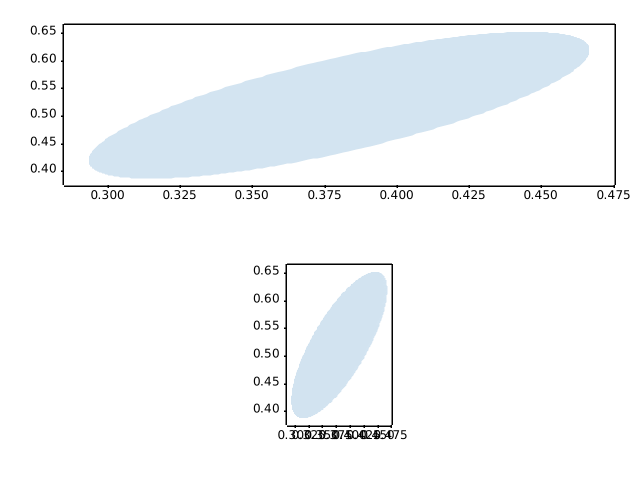
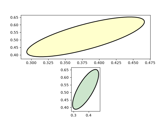
units/evans_test
==========
Source
"""
==========
Evans test
==========
A mockup "Foo" units class which supports conversion and different tick
formatting depending on the "unit". Here the "unit" is just a scalar
conversion factor, but this example shows that Matplotlib is entirely agnostic
to what kind of units client packages use.
"""
import matplotlib.pyplot as plt
import numpy as np
import matplotlib.ticker as ticker
import matplotlib.units as units
class Foo:
def __init__(self, val, unit=1.0):
self.unit = unit
self._val = val * unit
def value(self, unit):
if unit is None:
unit = self.unit
return self._val / unit
class FooConverter(units.ConversionInterface):
@staticmethod
def axisinfo(unit, axis):
"""Return the Foo AxisInfo."""
if unit == 1.0 or unit == 2.0:
return units.AxisInfo(
majloc=ticker.IndexLocator(8, 0),
majfmt=ticker.FormatStrFormatter("VAL: %s"),
label='foo',
)
else:
return None
@staticmethod
def convert(obj, unit, axis):
"""
Convert *obj* using *unit*.
If *obj* is a sequence, return the converted sequence.
"""
if np.iterable(obj):
return [o.value(unit) for o in obj]
else:
return obj.value(unit)
@staticmethod
def default_units(x, axis):
"""Return the default unit for *x* or None."""
if np.iterable(x):
for thisx in x:
return thisx.unit
else:
return x.unit
units.registry[Foo] = FooConverter()
# create some Foos
x = [Foo(val, 1.0) for val in range(0, 50, 2)]
# and some arbitrary y data
y = [i for i in range(len(x))]
fig, (ax1, ax2) = plt.subplots(1, 2)
fig.suptitle("Custom units")
fig.subplots_adjust(bottom=0.2)
# plot specifying units
ax2.plot(x, y, 'o', xunits=2.0)
ax2.set_title("xunits = 2.0")
ax2.tick_params(axis='x', rotation=30, rotation_mode='xtick')
# plot without specifying units; will use the None branch for axisinfo
ax1.plot(x, y) # uses default units
ax1.set_title('default units')
ax1.tick_params(axis='x', rotation=30, rotation_mode='xtick')
plt.show()
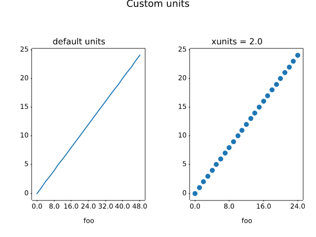
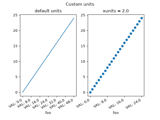
units/radian_demo
============
Source
""" ============ Radian ticks ============ Plot with radians from the basic_units mockup example package. This example shows how the unit class can determine the tick locating, formatting and axis labeling. .. only:: builder_html This example requires :download:`basic_units.py <basic_units.py>` """ from basic_units import cos, degrees, radians import matplotlib.pyplot as plt import numpy as np x = [val*radians for val in np.arange(0, 15, 0.01)] fig, axs = plt.subplots(2) axs[0].plot(x, cos(x), xunits=radians) axs[1].plot(x, cos(x), xunits=degrees) fig.tight_layout() plt.show()
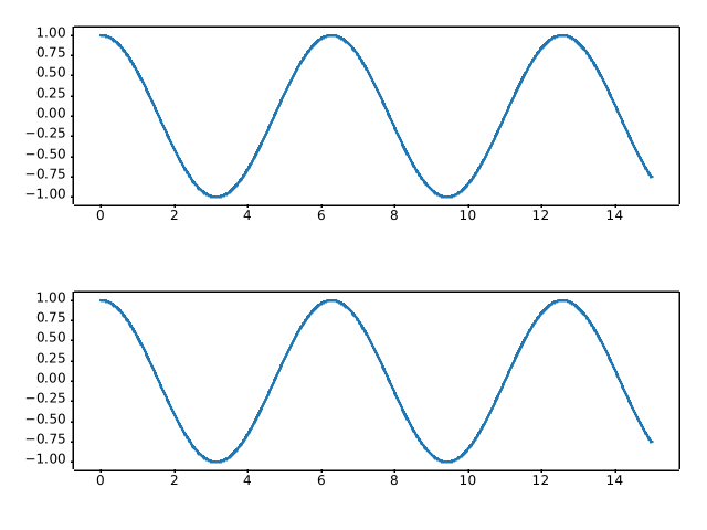
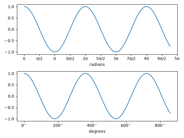
units/units_sample
======================
Source
""" ====================== Inches and centimeters ====================== The example illustrates the ability to override default x and y units (ax1) to inches and centimeters using the *xunits* and *yunits* parameters for the `~.axes.Axes.plot` function. Note that conversions are applied to get numbers to correct units. .. only:: builder_html This example requires :download:`basic_units.py <basic_units.py>` """ from basic_units import cm, inch import matplotlib.pyplot as plt import numpy as np cms = cm * np.arange(0, 10, 2) fig, axs = plt.subplots(2, 2, layout='constrained') axs[0, 0].plot(cms, cms) axs[0, 1].plot(cms, cms, xunits=cm, yunits=inch) axs[1, 0].plot(cms, cms, xunits=inch, yunits=cm) axs[1, 0].set_xlim(-1, 4) # scalars are interpreted in current units axs[1, 1].plot(cms, cms, xunits=inch, yunits=inch) axs[1, 1].set_xlim(3*cm, 6*cm) # cm are converted to inches plt.show()
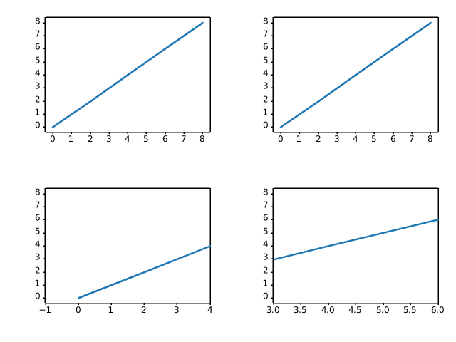
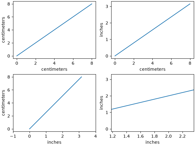
units/units_scatter
=============
Source
""" ============= Unit handling ============= The example below shows support for unit conversions over masked arrays. .. only:: builder_html This example requires :download:`basic_units.py <basic_units.py>` """ from basic_units import hertz, minutes, secs import matplotlib.pyplot as plt import numpy as np # create masked array data = (1, 2, 3, 4, 5, 6, 7, 8) mask = (1, 0, 1, 0, 0, 0, 1, 0) xsecs = secs * np.ma.MaskedArray(data, mask, float) fig, (ax1, ax2, ax3) = plt.subplots(nrows=3, sharex=True) ax1.scatter(xsecs, xsecs) ax1.yaxis.set_units(secs) ax2.scatter(xsecs, xsecs, yunits=hertz) ax3.scatter(xsecs, xsecs, yunits=minutes) fig.tight_layout() plt.show()
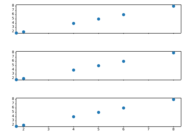
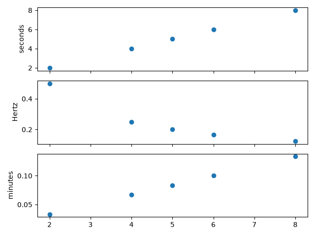
user_interfaces/canvasagg
==============
Source
"""
==============
CanvasAgg demo
==============
This example shows how to use the agg backend directly to create images, which
may be of use to web application developers who want full control over their
code without using the pyplot interface to manage figures, figure closing etc.
.. note::
It is not necessary to avoid using the pyplot interface in order to
create figures without a graphical front-end - simply setting
the backend to "Agg" would be sufficient.
In this example, we show how to save the contents of the agg canvas to a file,
and how to extract them to a numpy array, which can in turn be passed off
to Pillow_. The latter functionality allows e.g. to use Matplotlib inside a
cgi-script *without* needing to write a figure to disk, and to write images in
any format supported by Pillow.
.. _Pillow: https://pillow.readthedocs.io/
.. redirect-from:: /gallery/misc/agg_buffer
.. redirect-from:: /gallery/misc/agg_buffer_to_array
"""
# sphinx_gallery_thumbnail_path = '_static/canvasagg.png'
from PIL import Image
import numpy as np
from matplotlib.backends.backend_agg import FigureCanvasAgg
from matplotlib.figure import Figure
fig = Figure(figsize=(5, 4), dpi=100)
# Do some plotting.
ax = fig.add_subplot()
ax.plot([1, 2, 3])
# Option 1: Save the figure to a file; can also be a file-like object (BytesIO,
# etc.).
fig.savefig("test.png")
# Option 2 (low-level approach to directly save to a numpy array): Manually
# attach a canvas to the figure (pyplot or savefig would automatically do
# it), by instantiating the canvas with the figure as argument; then draw the
# figure, retrieve a memoryview on the renderer buffer, and convert it to a
# numpy array.
canvas = FigureCanvasAgg(fig)
canvas.draw()
rgba = np.asarray(canvas.buffer_rgba())
# ... and pass it to PIL.
im = Image.fromarray(rgba)
# This image can then be saved to any format supported by Pillow, e.g.:
im.save("test.bmp")
# Uncomment this line to display the image using ImageMagick's `display` tool.
# im.show()
# %%
#
# .. admonition:: References
#
# The use of the following functions, methods, classes and modules is shown
# in this example:
#
# - `matplotlib.backends.backend_agg.FigureCanvasAgg`
# - `matplotlib.figure.Figure`
# - `matplotlib.figure.Figure.add_subplot`
# - `matplotlib.figure.Figure.savefig` / `matplotlib.pyplot.savefig`
# - `matplotlib.axes.Axes.plot` / `matplotlib.pyplot.plot`
user_interfaces is out of scope
user_interfaces/embedding_in_gtk3_panzoom_sgskip
=======================================
Source
"""
=======================================
Embed in GTK3 with a navigation toolbar
=======================================
Demonstrate NavigationToolbar with GTK3 accessed via pygobject.
"""
import gi
gi.require_version('Gtk', '3.0')
from gi.repository import Gtk
import numpy as np
from matplotlib.backends.backend_gtk3 import NavigationToolbar2GTK3 as NavigationToolbar
from matplotlib.backends.backend_gtk3agg import FigureCanvasGTK3Agg as FigureCanvas
from matplotlib.figure import Figure
win = Gtk.Window()
win.connect("delete-event", Gtk.main_quit)
win.set_default_size(400, 300)
win.set_title("Embedded in GTK3")
fig = Figure(figsize=(5, 4), dpi=100)
ax = fig.add_subplot(1, 1, 1)
t = np.arange(0.0, 3.0, 0.01)
s = np.sin(2*np.pi*t)
ax.plot(t, s)
vbox = Gtk.VBox()
win.add(vbox)
# Add canvas to vbox
canvas = FigureCanvas(fig) # a Gtk.DrawingArea
vbox.pack_start(canvas, True, True, 0)
# Create toolbar
toolbar = NavigationToolbar(canvas)
vbox.pack_start(toolbar, False, False, 0)
win.show_all()
Gtk.main()
user_interfaces is out of scope
user_interfaces/embedding_in_gtk3_sgskip
=============
Source
"""
=============
Embed in GTK3
=============
Demonstrate adding a FigureCanvasGTK3Agg widget to a Gtk.ScrolledWindow using
GTK3 accessed via pygobject.
"""
import gi
gi.require_version('Gtk', '3.0')
from gi.repository import Gtk
import numpy as np
from matplotlib.backends.backend_gtk3agg import FigureCanvasGTK3Agg as FigureCanvas
from matplotlib.figure import Figure
win = Gtk.Window()
win.connect("delete-event", Gtk.main_quit)
win.set_default_size(400, 300)
win.set_title("Embedded in GTK3")
fig = Figure(figsize=(5, 4), dpi=100)
ax = fig.add_subplot()
t = np.arange(0.0, 3.0, 0.01)
s = np.sin(2*np.pi*t)
ax.plot(t, s)
sw = Gtk.ScrolledWindow()
win.add(sw)
# A scrolled window border goes outside the scrollbars and viewport
sw.set_border_width(10)
canvas = FigureCanvas(fig) # a Gtk.DrawingArea
canvas.set_size_request(800, 600)
sw.add(canvas)
win.show_all()
Gtk.main()
user_interfaces is out of scope
user_interfaces/embedding_in_gtk4_panzoom_sgskip
=======================================
Source
"""
=======================================
Embed in GTK4 with a navigation toolbar
=======================================
Demonstrate NavigationToolbar with GTK4 accessed via pygobject.
"""
import gi
gi.require_version('Gtk', '4.0')
from gi.repository import Gtk
import numpy as np
from matplotlib.backends.backend_gtk4 import NavigationToolbar2GTK4 as NavigationToolbar
from matplotlib.backends.backend_gtk4agg import FigureCanvasGTK4Agg as FigureCanvas
from matplotlib.figure import Figure
def on_activate(app):
win = Gtk.ApplicationWindow(application=app)
win.set_default_size(400, 300)
win.set_title("Embedded in GTK4")
fig = Figure(figsize=(5, 4), dpi=100)
ax = fig.add_subplot(1, 1, 1)
t = np.arange(0.0, 3.0, 0.01)
s = np.sin(2*np.pi*t)
ax.plot(t, s)
vbox = Gtk.Box(orientation=Gtk.Orientation.VERTICAL)
win.set_child(vbox)
# Add canvas to vbox
canvas = FigureCanvas(fig) # a Gtk.DrawingArea
canvas.set_hexpand(True)
canvas.set_vexpand(True)
vbox.append(canvas)
# Create toolbar
toolbar = NavigationToolbar(canvas)
vbox.append(toolbar)
win.present()
app = Gtk.Application(application_id='org.matplotlib.examples.EmbeddingInGTK4PanZoom')
app.connect('activate', on_activate)
app.run(None)
user_interfaces is out of scope
user_interfaces/embedding_in_gtk4_sgskip
=============
Source
"""
=============
Embed in GTK4
=============
Demonstrate adding a FigureCanvasGTK4Agg widget to a Gtk.ScrolledWindow using
GTK4 accessed via pygobject.
"""
import gi
gi.require_version('Gtk', '4.0')
from gi.repository import Gtk
import numpy as np
from matplotlib.backends.backend_gtk4agg import FigureCanvasGTK4Agg as FigureCanvas
from matplotlib.figure import Figure
def on_activate(app):
win = Gtk.ApplicationWindow(application=app)
win.set_default_size(400, 300)
win.set_title("Embedded in GTK4")
fig = Figure(figsize=(5, 4), dpi=100)
ax = fig.add_subplot()
t = np.arange(0.0, 3.0, 0.01)
s = np.sin(2*np.pi*t)
ax.plot(t, s)
# A scrolled margin goes outside the scrollbars and viewport.
sw = Gtk.ScrolledWindow(margin_top=10, margin_bottom=10,
margin_start=10, margin_end=10)
win.set_child(sw)
canvas = FigureCanvas(fig) # a Gtk.DrawingArea
canvas.set_size_request(800, 600)
sw.set_child(canvas)
win.present()
app = Gtk.Application(application_id='org.matplotlib.examples.EmbeddingInGTK4')
app.connect('activate', on_activate)
app.run(None)
user_interfaces is out of scope
user_interfaces/embedding_in_qt_sgskip
===========
Source
"""
===========
Embed in Qt
===========
Simple Qt application embedding Matplotlib canvases. This program will work
equally well using any Qt binding (PyQt6, PySide6, PyQt5, PySide2). The
binding can be selected by setting the :envvar:`QT_API` environment variable to
the binding name, or by first importing it.
"""
# sphinx_gallery_thumbnail_path = '_static/embedding_in_qt.png'
import sys
import time
import numpy as np
from matplotlib.backends.backend_qtagg import FigureCanvas
from matplotlib.backends.backend_qtagg import NavigationToolbar2QT as NavigationToolbar
from matplotlib.backends.qt_compat import QtWidgets
from matplotlib.figure import Figure
class ApplicationWindow(QtWidgets.QMainWindow):
def __init__(self):
super().__init__()
self._main = QtWidgets.QWidget()
self.setCentralWidget(self._main)
layout = QtWidgets.QVBoxLayout(self._main)
static_canvas = FigureCanvas(Figure(figsize=(5, 3)))
# Ideally one would use self.addToolBar here, but it is slightly
# incompatible between PyQt6 and other bindings, so we just add the
# toolbar as a plain widget instead.
layout.addWidget(NavigationToolbar(static_canvas, self))
layout.addWidget(static_canvas)
dynamic_canvas = FigureCanvas(Figure(figsize=(5, 3)))
layout.addWidget(dynamic_canvas)
layout.addWidget(NavigationToolbar(dynamic_canvas, self))
self._static_ax = static_canvas.figure.subplots()
t = np.linspace(0, 10, 501)
self._static_ax.plot(t, np.tan(t), ".")
self._dynamic_ax = dynamic_canvas.figure.subplots()
# Set up a Line2D.
self.xdata = np.linspace(0, 10, 101)
self._update_ydata()
self._line, = self._dynamic_ax.plot(self.xdata, self.ydata)
# The below two timers must be attributes of self, so that the garbage
# collector won't clean them after we finish with __init__...
# The data retrieval may be fast as possible (Using QRunnable could be
# even faster).
self.data_timer = dynamic_canvas.new_timer(1)
self.data_timer.add_callback(self._update_ydata)
self.data_timer.start()
# Drawing at 50Hz should be fast enough for the GUI to feel smooth, and
# not too fast for the GUI to be overloaded with events that need to be
# processed while the GUI element is changed.
self.drawing_timer = dynamic_canvas.new_timer(20)
self.drawing_timer.add_callback(self._update_canvas)
self.drawing_timer.start()
def _update_ydata(self):
# Shift the sinusoid as a function of time.
self.ydata = np.sin(self.xdata + time.time())
def _update_canvas(self):
self._line.set_data(self.xdata, self.ydata)
# It should be safe to use the synchronous draw() method for most drawing
# frequencies, but it is safer to use draw_idle().
self._line.figure.canvas.draw_idle()
if __name__ == "__main__":
# Check whether there is already a running QApplication (e.g., if running
# from an IDE).
qapp = QtWidgets.QApplication.instance()
if not qapp:
qapp = QtWidgets.QApplication(sys.argv)
app = ApplicationWindow()
app.show()
app.activateWindow()
app.raise_()
qapp.exec()
user_interfaces is out of scope
user_interfaces/embedding_in_tk_sgskip
===========
Source
"""
===========
Embed in Tk
===========
"""
# sphinx_gallery_thumbnail_path = '_static/embedding_in_tk.png'
import tkinter
import numpy as np
# Implement the default Matplotlib key bindings.
from matplotlib.backend_bases import key_press_handler
from matplotlib.backends.backend_tkagg import FigureCanvasTkAgg, NavigationToolbar2Tk
from matplotlib.figure import Figure
root = tkinter.Tk()
root.wm_title("Embedded in Tk")
fig = Figure(figsize=(5, 4), dpi=100)
t = np.arange(0, 3, .01)
ax = fig.add_subplot()
line, = ax.plot(t, 2 * np.sin(2 * np.pi * t))
ax.set_xlabel("time [s]")
ax.set_ylabel("f(t)")
canvas = FigureCanvasTkAgg(fig, master=root) # A tk.DrawingArea.
canvas.draw()
# pack_toolbar=False will make it easier to use a layout manager later on.
toolbar = NavigationToolbar2Tk(canvas, root, pack_toolbar=False)
toolbar.update()
canvas.mpl_connect(
"key_press_event", lambda event: print(f"you pressed {event.key}"))
canvas.mpl_connect("key_press_event", key_press_handler)
button_quit = tkinter.Button(master=root, text="Quit", command=root.destroy)
def update_frequency(new_val):
# retrieve frequency
f = float(new_val)
# update data
y = 2 * np.sin(2 * np.pi * f * t)
line.set_data(t, y)
# required to update canvas and attached toolbar!
canvas.draw()
slider_update = tkinter.Scale(root, from_=1, to=5, orient=tkinter.HORIZONTAL,
command=update_frequency, label="Frequency [Hz]")
# Packing order is important. Widgets are processed sequentially and if there
# is no space left, because the window is too small, they are not displayed.
# The canvas is rather flexible in its size, so we pack it last which makes
# sure the UI controls are displayed as long as possible.
button_quit.pack(side=tkinter.BOTTOM)
slider_update.pack(side=tkinter.BOTTOM)
toolbar.pack(side=tkinter.BOTTOM, fill=tkinter.X)
canvas.get_tk_widget().pack(side=tkinter.TOP, fill=tkinter.BOTH, expand=True)
tkinter.mainloop()
user_interfaces is out of scope
user_interfaces/embedding_in_wx2_sgskip
==============
Source
"""
==============
Embed in wx #2
==============
An example of how to use wxagg in an application with the new
toolbar - comment out the add_toolbar line for no toolbar.
"""
import wx
import wx.lib.mixins.inspection as WIT
import numpy as np
from matplotlib.backends.backend_wxagg import FigureCanvasWxAgg as FigureCanvas
from matplotlib.backends.backend_wxagg import \
NavigationToolbar2WxAgg as NavigationToolbar
from matplotlib.figure import Figure
class CanvasFrame(wx.Frame):
def __init__(self):
super().__init__(None, -1, 'CanvasFrame', size=(550, 350))
self.figure = Figure()
self.axes = self.figure.add_subplot()
t = np.arange(0.0, 3.0, 0.01)
s = np.sin(2 * np.pi * t)
self.axes.plot(t, s)
self.canvas = FigureCanvas(self, -1, self.figure)
self.sizer = wx.BoxSizer(wx.VERTICAL)
self.sizer.Add(self.canvas, 1, wx.LEFT | wx.TOP | wx.EXPAND)
self.SetSizer(self.sizer)
self.Fit()
self.add_toolbar() # comment this out for no toolbar
def add_toolbar(self):
self.toolbar = NavigationToolbar(self.canvas)
self.toolbar.Realize()
# By adding toolbar in sizer, we are able to put it at the bottom
# of the frame - so appearance is closer to GTK version.
self.sizer.Add(self.toolbar, 0, wx.LEFT | wx.EXPAND)
# update the axes menu on the toolbar
self.toolbar.update()
# Alternatively you could use:
# class App(wx.App):
class App(WIT.InspectableApp):
def OnInit(self):
"""Create the main window and insert the custom frame."""
self.Init()
frame = CanvasFrame()
frame.Show(True)
return True
if __name__ == "__main__":
app = App()
app.MainLoop()
user_interfaces is out of scope
user_interfaces/embedding_in_wx3_sgskip
==============
Source
"""
==============
Embed in wx #3
==============
Copyright (C) 2003-2004 Andrew Straw, Jeremy O'Donoghue and others
License: This work is licensed under the PSF. A copy should be included
with this source code, and is also available at
https://docs.python.org/3/license.html
This is yet another example of using matplotlib with wx. Hopefully
this is pretty full-featured:
- both matplotlib toolbar and WX buttons manipulate plot
- full wxApp framework, including widget interaction
- XRC (XML wxWidgets resource) file to create GUI (made with XRCed)
This was derived from embedding_in_wx and dynamic_image_wxagg.
Thanks to matplotlib and wx teams for creating such great software!
"""
import wx
import wx.xrc as xrc
import numpy as np
from matplotlib.backends.backend_wxagg import FigureCanvasWxAgg as FigureCanvas
from matplotlib.backends.backend_wxagg import \
NavigationToolbar2WxAgg as NavigationToolbar
import matplotlib.cbook as cbook
from matplotlib.figure import Figure
ERR_TOL = 1e-5 # floating point slop for peak-detection
class PlotPanel(wx.Panel):
def __init__(self, parent):
super().__init__(parent, -1)
self.fig = Figure((5, 4), 75)
self.canvas = FigureCanvas(self, -1, self.fig)
self.toolbar = NavigationToolbar(self.canvas) # matplotlib toolbar
self.toolbar.Realize()
# Now put all into a sizer
sizer = wx.BoxSizer(wx.VERTICAL)
# This way of adding to sizer allows resizing
sizer.Add(self.canvas, 1, wx.LEFT | wx.TOP | wx.GROW)
# Best to allow the toolbar to resize!
sizer.Add(self.toolbar, 0, wx.GROW)
self.SetSizer(sizer)
self.Fit()
def init_plot_data(self):
ax = self.fig.add_subplot()
x = np.arange(120.0) * 2 * np.pi / 60.0
y = np.arange(100.0) * 2 * np.pi / 50.0
self.x, self.y = np.meshgrid(x, y)
z = np.sin(self.x) + np.cos(self.y)
self.im = ax.imshow(z, cmap="RdBu", origin='lower')
zmax = np.max(z) - ERR_TOL
ymax_i, xmax_i = np.nonzero(z >= zmax)
if self.im.origin == 'upper':
ymax_i = z.shape[0] - ymax_i
self.lines = ax.plot(xmax_i, ymax_i, 'ko')
self.toolbar.update() # Not sure why this is needed - ADS
def GetToolBar(self):
# You will need to override GetToolBar if you are using an
# unmanaged toolbar in your frame
return self.toolbar
def OnWhiz(self, event):
self.x += np.pi / 15
self.y += np.pi / 20
z = np.sin(self.x) + np.cos(self.y)
self.im.set_array(z)
zmax = np.max(z) - ERR_TOL
ymax_i, xmax_i = np.nonzero(z >= zmax)
if self.im.origin == 'upper':
ymax_i = z.shape[0] - ymax_i
self.lines[0].set_data(xmax_i, ymax_i)
self.canvas.draw()
class MyApp(wx.App):
def OnInit(self):
xrcfile = cbook.get_sample_data('embedding_in_wx3.xrc',
asfileobj=False)
print('loading', xrcfile)
self.res = xrc.XmlResource(xrcfile)
# main frame and panel ---------
self.frame = self.res.LoadFrame(None, "MainFrame")
self.panel = xrc.XRCCTRL(self.frame, "MainPanel")
# matplotlib panel -------------
# container for matplotlib panel (I like to make a container
# panel for our panel so I know where it'll go when in XRCed.)
plot_container = xrc.XRCCTRL(self.frame, "plot_container_panel")
sizer = wx.BoxSizer(wx.VERTICAL)
# matplotlib panel itself
self.plotpanel = PlotPanel(plot_container)
self.plotpanel.init_plot_data()
# wx boilerplate
sizer.Add(self.plotpanel, 1, wx.EXPAND)
plot_container.SetSizer(sizer)
# whiz button ------------------
whiz_button = xrc.XRCCTRL(self.frame, "whiz_button")
whiz_button.Bind(wx.EVT_BUTTON, self.plotpanel.OnWhiz)
# bang button ------------------
bang_button = xrc.XRCCTRL(self.frame, "bang_button")
bang_button.Bind(wx.EVT_BUTTON, self.OnBang)
# final setup ------------------
self.frame.Show()
self.SetTopWindow(self.frame)
return True
def OnBang(self, event):
bang_count = xrc.XRCCTRL(self.frame, "bang_count")
bangs = bang_count.GetValue()
bangs = int(bangs) + 1
bang_count.SetValue(str(bangs))
if __name__ == '__main__':
app = MyApp()
app.MainLoop()
user_interfaces is out of scope
user_interfaces/embedding_in_wx4_sgskip
==============
Source
"""
==============
Embed in wx #4
==============
An example of how to use wxagg in a wx application with a custom toolbar.
"""
import wx
import numpy as np
from matplotlib.backends.backend_wxagg import FigureCanvasWxAgg as FigureCanvas
from matplotlib.backends.backend_wxagg import \
NavigationToolbar2WxAgg as NavigationToolbar
from matplotlib.figure import Figure
class MyNavigationToolbar(NavigationToolbar):
"""Extend the default wx toolbar with your own event handlers."""
def __init__(self, canvas):
super().__init__(canvas)
# We use a stock wx bitmap, but you could also use your own image file.
bmp = wx.ArtProvider.GetBitmap(wx.ART_CROSS_MARK, wx.ART_TOOLBAR)
tool = self.AddTool(wx.ID_ANY, 'Click me', bmp,
'Activate custom control')
self.Bind(wx.EVT_TOOL, self._on_custom, id=tool.GetId())
def _on_custom(self, event):
# add some text to the Axes in a random location in axes coords with a
# random color
ax = self.canvas.figure.axes[0]
x, y = np.random.rand(2) # generate a random location
rgb = np.random.rand(3) # generate a random color
ax.text(x, y, 'You clicked me', transform=ax.transAxes, color=rgb)
self.canvas.draw()
event.Skip()
class CanvasFrame(wx.Frame):
def __init__(self):
super().__init__(None, -1, 'CanvasFrame', size=(550, 350))
self.figure = Figure(figsize=(5, 4), dpi=100)
self.axes = self.figure.add_subplot()
t = np.arange(0.0, 3.0, 0.01)
s = np.sin(2 * np.pi * t)
self.axes.plot(t, s)
self.canvas = FigureCanvas(self, -1, self.figure)
self.sizer = wx.BoxSizer(wx.VERTICAL)
self.sizer.Add(self.canvas, 1, wx.TOP | wx.LEFT | wx.EXPAND)
self.toolbar = MyNavigationToolbar(self.canvas)
self.toolbar.Realize()
# By adding toolbar in sizer, we are able to put it at the bottom
# of the frame - so appearance is closer to GTK version.
self.sizer.Add(self.toolbar, 0, wx.LEFT | wx.EXPAND)
# update the axes menu on the toolbar
self.toolbar.update()
self.SetSizer(self.sizer)
self.Fit()
class App(wx.App):
def OnInit(self):
"""Create the main window and insert the custom frame."""
frame = CanvasFrame()
frame.Show(True)
return True
if __name__ == "__main__":
app = App()
app.MainLoop()
user_interfaces is out of scope
user_interfaces/embedding_in_wx5_sgskip
==============
Source
"""
==============
Embed in wx #5
==============
.. tip::
As a development and debugging aid, you can replace :class:`wx.App`
by :class:`wx.lib.mixins.inspection.InspectableApp`.
This adds the capability to start the `Widget Inspection Tool
<https://wiki.wxpython.org/How%20to%20use%20Widget%20Inspection%20Tool%20-%20WIT%20%28Phoenix%29>`_
via :kbd:`Ctrl-Alt-I`.
"""
import wx
import wx.lib.agw.aui as aui
from matplotlib.backends.backend_wxagg import FigureCanvasWxAgg as FigureCanvas
from matplotlib.backends.backend_wxagg import \
NavigationToolbar2WxAgg as NavigationToolbar
from matplotlib.figure import Figure
class Plot(wx.Panel):
def __init__(self, parent, id=-1, dpi=None, **kwargs):
super().__init__(parent, id=id, **kwargs)
self.figure = Figure(dpi=dpi, figsize=(2, 2))
self.canvas = FigureCanvas(self, -1, self.figure)
self.toolbar = NavigationToolbar(self.canvas)
self.toolbar.Realize()
sizer = wx.BoxSizer(wx.VERTICAL)
sizer.Add(self.canvas, 1, wx.EXPAND)
sizer.Add(self.toolbar, 0, wx.LEFT | wx.EXPAND)
self.SetSizer(sizer)
class PlotNotebook(wx.Panel):
def __init__(self, parent, id=-1):
super().__init__(parent, id=id)
self.nb = aui.AuiNotebook(self)
sizer = wx.BoxSizer()
sizer.Add(self.nb, 1, wx.EXPAND)
self.SetSizer(sizer)
def add(self, name="plot"):
page = Plot(self.nb)
self.nb.AddPage(page, name)
return page.figure
def demo():
app = wx.App()
frame = wx.Frame(None, -1, 'Plotter')
plotter = PlotNotebook(frame)
axes1 = plotter.add('figure 1').add_subplot()
axes1.plot([1, 2, 3], [2, 1, 4])
axes2 = plotter.add('figure 2').add_subplot()
axes2.plot([1, 2, 3, 4, 5], [2, 1, 4, 2, 3])
frame.Show()
app.MainLoop()
if __name__ == "__main__":
demo()
user_interfaces is out of scope
user_interfaces/embedding_webagg_sgskip
================
Source
"""
================
Embedding WebAgg
================
This example demonstrates how to embed Matplotlib WebAgg interactive plotting
in your own web application and framework. It is not necessary to do all this
if you merely want to display a plot in a browser or use Matplotlib's built-in
Tornado-based server "on the side".
The framework being used must support web sockets.
"""
# sphinx_gallery_thumbnail_path = '_static/embedding_webagg.png'
import argparse
import io
import json
import mimetypes
from pathlib import Path
import signal
import socket
try:
import tornado
except ImportError as err:
raise RuntimeError("This example requires tornado.") from err
import tornado.httpserver
import tornado.ioloop
import tornado.web
import tornado.websocket
import numpy as np
import matplotlib as mpl
from matplotlib.backends.backend_webagg import (FigureManagerWebAgg,
new_figure_manager_given_figure)
from matplotlib.figure import Figure
def create_figure():
"""
Creates a simple example figure.
"""
fig = Figure()
ax = fig.add_subplot()
t = np.arange(0.0, 3.0, 0.01)
s = np.sin(2 * np.pi * t)
ax.plot(t, s)
return fig
# The following is the content of the web page. You would normally
# generate this using some sort of template facility in your web
# framework, but here we just use Python string formatting.
html_content = """<!DOCTYPE html>
<html lang="en">
<head>
<!-- TODO: There should be a way to include all of the required javascript
and CSS so matplotlib can add to the set in the future if it
needs to. -->
<link rel="stylesheet" href="_static/css/page.css" type="text/css">
<link rel="stylesheet" href="_static/css/boilerplate.css" type="text/css">
<link rel="stylesheet" href="_static/css/fbm.css" type="text/css">
<link rel="stylesheet" href="_static/css/mpl.css" type="text/css">
<script src="mpl.js"></script>
<script>
/* This is a callback that is called when the user saves
(downloads) a file. Its purpose is really to map from a
figure and file format to a url in the application. */
function ondownload(figure, format) {
window.open('download.' + format, '_blank');
};
function ready(fn) {
if (document.readyState != "loading") {
fn();
} else {
document.addEventListener("DOMContentLoaded", fn);
}
}
ready(
function() {
/* It is up to the application to provide a websocket that the figure
will use to communicate to the server. This websocket object can
also be a "fake" websocket that underneath multiplexes messages
from multiple figures, if necessary. */
var websocket_type = mpl.get_websocket_type();
var websocket = new websocket_type("%(ws_uri)sws");
// mpl.figure creates a new figure on the webpage.
var fig = new mpl.figure(
// A unique numeric identifier for the figure
%(fig_id)s,
// A websocket object (or something that behaves like one)
websocket,
// A function called when a file type is selected for download
ondownload,
// The HTML element in which to place the figure
document.getElementById("figure"));
}
);
</script>
<title>matplotlib</title>
</head>
<body>
<div id="figure">
</div>
</body>
</html>
"""
class MyApplication(tornado.web.Application):
class MainPage(tornado.web.RequestHandler):
"""
Serves the main HTML page.
"""
def get(self):
manager = self.application.manager
ws_uri = f"ws://{self.request.host}/"
content = html_content % {
"ws_uri": ws_uri, "fig_id": manager.num}
self.write(content)
class MplJs(tornado.web.RequestHandler):
"""
Serves the generated matplotlib javascript file. The content
is dynamically generated based on which toolbar functions the
user has defined. Call `FigureManagerWebAgg` to get its
content.
"""
def get(self):
self.set_header('Content-Type', 'application/javascript')
js_content = FigureManagerWebAgg.get_javascript()
self.write(js_content)
class Download(tornado.web.RequestHandler):
"""
Handles downloading of the figure in various file formats.
"""
def get(self, fmt):
manager = self.application.manager
self.set_header(
'Content-Type', mimetypes.types_map.get(fmt, 'binary'))
buff = io.BytesIO()
manager.canvas.figure.savefig(buff, format=fmt)
self.write(buff.getvalue())
class WebSocket(tornado.websocket.WebSocketHandler):
"""
A websocket for interactive communication between the plot in
the browser and the server.
In addition to the methods required by tornado, it is required to
have two callback methods:
- ``send_json(json_content)`` is called by matplotlib when
it needs to send json to the browser. `json_content` is
a JSON tree (Python dictionary), and it is the responsibility
of this implementation to encode it as a string to send over
the socket.
- ``send_binary(blob)`` is called to send binary image data
to the browser.
"""
supports_binary = True
def open(self):
# Register the websocket with the FigureManager.
manager = self.application.manager
manager.add_web_socket(self)
if hasattr(self, 'set_nodelay'):
self.set_nodelay(True)
def on_close(self):
# When the socket is closed, deregister the websocket with
# the FigureManager.
manager = self.application.manager
manager.remove_web_socket(self)
def on_message(self, message):
# The 'supports_binary' message is relevant to the
# websocket itself. The other messages get passed along
# to matplotlib as-is.
# Every message has a "type" and a "figure_id".
message = json.loads(message)
if message['type'] == 'supports_binary':
self.supports_binary = message['value']
else:
manager = self.application.manager
manager.handle_json(message)
def send_json(self, content):
self.write_message(json.dumps(content))
def send_binary(self, blob):
if self.supports_binary:
self.write_message(blob, binary=True)
else:
data_uri = ("data:image/png;base64," +
blob.encode('base64').replace('\n', ''))
self.write_message(data_uri)
def __init__(self, figure):
self.figure = figure
self.manager = new_figure_manager_given_figure(id(figure), figure)
super().__init__([
# Static files for the CSS and JS
(r'/_static/(.*)',
tornado.web.StaticFileHandler,
{'path': FigureManagerWebAgg.get_static_file_path()}),
# Static images for the toolbar
(r'/_images/(.*)',
tornado.web.StaticFileHandler,
{'path': Path(mpl.get_data_path(), 'images')}),
# The page that contains all of the pieces
('/', self.MainPage),
('/mpl.js', self.MplJs),
# Sends images and events to the browser, and receives
# events from the browser
('/ws', self.WebSocket),
# Handles the downloading (i.e., saving) of static images
(r'/download.([a-z0-9.]+)', self.Download),
])
if __name__ == "__main__":
parser = argparse.ArgumentParser()
parser.add_argument('-p', '--port', type=int, default=8080,
help='Port to listen on (0 for a random port).')
args = parser.parse_args()
figure = create_figure()
application = MyApplication(figure)
http_server = tornado.httpserver.HTTPServer(application)
sockets = tornado.netutil.bind_sockets(args.port, '')
http_server.add_sockets(sockets)
for s in sockets:
addr, port = s.getsockname()[:2]
if s.family is socket.AF_INET6:
addr = f'[{addr}]'
print(f"Listening on http://{addr}:{port}/")
print("Press Ctrl+C to quit")
ioloop = tornado.ioloop.IOLoop.instance()
def shutdown():
ioloop.stop()
print("Server stopped")
old_handler = signal.signal(
signal.SIGINT,
lambda sig, frame: ioloop.add_callback_from_signal(shutdown))
try:
ioloop.start()
finally:
signal.signal(signal.SIGINT, old_handler)
user_interfaces is out of scope
user_interfaces/fourier_demo_wx_sgskip
===============
Source
"""
===============
Fourier Demo WX
===============
"""
import wx
import numpy as np
from matplotlib.backends.backend_wxagg import FigureCanvasWxAgg as FigureCanvas
from matplotlib.figure import Figure
class Knob:
"""
Knob - simple class with a "setKnob" method.
A Knob instance is attached to a Param instance, e.g., param.attach(knob)
Base class is for documentation purposes.
"""
def setKnob(self, value):
pass
class Param:
"""
The idea of the "Param" class is that some parameter in the GUI may have
several knobs that both control it and reflect the parameter's state, e.g.
a slider, text, and dragging can all change the value of the frequency in
the waveform of this example.
The class allows a cleaner way to update/"feedback" to the other knobs when
one is being changed. Also, this class handles min/max constraints for all
the knobs.
Idea - knob list - in "set" method, knob object is passed as well
- the other knobs in the knob list have a "set" method which gets
called for the others.
"""
def __init__(self, initialValue=None, minimum=0., maximum=1.):
self.minimum = minimum
self.maximum = maximum
if initialValue != self.constrain(initialValue):
raise ValueError('illegal initial value')
self.value = initialValue
self.knobs = []
def attach(self, knob):
self.knobs += [knob]
def set(self, value, knob=None):
self.value = value
self.value = self.constrain(value)
for feedbackKnob in self.knobs:
if feedbackKnob != knob:
feedbackKnob.setKnob(self.value)
return self.value
def constrain(self, value):
if value <= self.minimum:
value = self.minimum
if value >= self.maximum:
value = self.maximum
return value
class SliderGroup(Knob):
def __init__(self, parent, label, param):
self.sliderLabel = wx.StaticText(parent, label=label)
self.sliderText = wx.TextCtrl(parent, -1, style=wx.TE_PROCESS_ENTER)
self.slider = wx.Slider(parent, -1)
# self.slider.SetMax(param.maximum*1000)
self.slider.SetRange(0, int(param.maximum * 1000))
self.setKnob(param.value)
sizer = wx.BoxSizer(wx.HORIZONTAL)
sizer.Add(self.sliderLabel, 0,
wx.EXPAND | wx.ALL,
border=2)
sizer.Add(self.sliderText, 0,
wx.EXPAND | wx.ALL,
border=2)
sizer.Add(self.slider, 1, wx.EXPAND)
self.sizer = sizer
self.slider.Bind(wx.EVT_SLIDER, self.sliderHandler)
self.sliderText.Bind(wx.EVT_TEXT_ENTER, self.sliderTextHandler)
self.param = param
self.param.attach(self)
def sliderHandler(self, event):
value = event.GetInt() / 1000.
self.param.set(value)
def sliderTextHandler(self, event):
value = float(self.sliderText.GetValue())
self.param.set(value)
def setKnob(self, value):
self.sliderText.SetValue(f'{value:g}')
self.slider.SetValue(int(value * 1000))
class FourierDemoFrame(wx.Frame):
def __init__(self, *args, **kwargs):
super().__init__(*args, **kwargs)
panel = wx.Panel(self)
# create the GUI elements
self.createCanvas(panel)
self.createSliders(panel)
# place them in a sizer for the Layout
sizer = wx.BoxSizer(wx.VERTICAL)
sizer.Add(self.canvas, 1, wx.EXPAND)
sizer.Add(self.frequencySliderGroup.sizer, 0,
wx.EXPAND | wx.ALL, border=5)
sizer.Add(self.amplitudeSliderGroup.sizer, 0,
wx.EXPAND | wx.ALL, border=5)
panel.SetSizer(sizer)
def createCanvas(self, parent):
self.lines = []
self.figure = Figure()
self.canvas = FigureCanvas(parent, -1, self.figure)
self.canvas.callbacks.connect('button_press_event', self.mouseDown)
self.canvas.callbacks.connect('motion_notify_event', self.mouseMotion)
self.canvas.callbacks.connect('button_release_event', self.mouseUp)
self.state = ''
self.mouseInfo = (None, None, None, None)
self.f0 = Param(2., minimum=0., maximum=6.)
self.A = Param(1., minimum=0.01, maximum=2.)
self.createPlots()
# Not sure I like having two params attached to the same Knob,
# but that is what we have here... it works but feels kludgy -
# although maybe it's not too bad since the knob changes both params
# at the same time (both f0 and A are affected during a drag)
self.f0.attach(self)
self.A.attach(self)
def createSliders(self, panel):
self.frequencySliderGroup = SliderGroup(
panel,
label='Frequency f0:',
param=self.f0)
self.amplitudeSliderGroup = SliderGroup(panel, label=' Amplitude a:',
param=self.A)
def mouseDown(self, event):
if self.lines[0].contains(event)[0]:
self.state = 'frequency'
elif self.lines[1].contains(event)[0]:
self.state = 'time'
else:
self.state = ''
self.mouseInfo = (event.xdata, event.ydata,
max(self.f0.value, .1),
self.A.value)
def mouseMotion(self, event):
if self.state == '':
return
x, y = event.xdata, event.ydata
if x is None: # outside the Axes
return
x0, y0, f0Init, AInit = self.mouseInfo
self.A.set(AInit + (AInit * (y - y0) / y0), self)
if self.state == 'frequency':
self.f0.set(f0Init + (f0Init * (x - x0) / x0))
elif self.state == 'time':
if (x - x0) / x0 != -1.:
self.f0.set(1. / (1. / f0Init + (1. / f0Init * (x - x0) / x0)))
def mouseUp(self, event):
self.state = ''
def createPlots(self):
# This method creates the subplots, waveforms and labels.
# Later, when the waveforms or sliders are dragged, only the
# waveform data will be updated (not here, but below in setKnob).
self.subplot1, self.subplot2 = self.figure.subplots(2)
x1, y1, x2, y2 = self.compute(self.f0.value, self.A.value)
color = (1., 0., 0.)
self.lines += self.subplot1.plot(x1, y1, color=color, linewidth=2)
self.lines += self.subplot2.plot(x2, y2, color=color, linewidth=2)
# Set some plot attributes
self.subplot1.set_title(
"Click and drag waveforms to change frequency and amplitude",
fontsize=12)
self.subplot1.set_ylabel("Frequency Domain Waveform X(f)", fontsize=8)
self.subplot1.set_xlabel("frequency f", fontsize=8)
self.subplot2.set_ylabel("Time Domain Waveform x(t)", fontsize=8)
self.subplot2.set_xlabel("time t", fontsize=8)
self.subplot1.set_xlim(-6, 6)
self.subplot1.set_ylim(0, 1)
self.subplot2.set_xlim(-2, 2)
self.subplot2.set_ylim(-2, 2)
self.subplot1.text(0.05, .95,
r'$X(f) = \mathcal{F}\{x(t)\}$',
verticalalignment='top',
transform=self.subplot1.transAxes)
self.subplot2.text(0.05, .95,
r'$x(t) = a \cdot \cos(2\pi f_0 t) e^{-\pi t^2}$',
verticalalignment='top',
transform=self.subplot2.transAxes)
def compute(self, f0, A):
f = np.arange(-6., 6., 0.02)
t = np.arange(-2., 2., 0.01)
x = A * np.cos(2 * np.pi * f0 * t) * np.exp(-np.pi * t ** 2)
X = A / 2 * \
(np.exp(-np.pi * (f - f0) ** 2) + np.exp(-np.pi * (f + f0) ** 2))
return f, X, t, x
def setKnob(self, value):
# Note, we ignore value arg here and just go by state of the params
x1, y1, x2, y2 = self.compute(self.f0.value, self.A.value)
# update the data of the two waveforms
self.lines[0].set(xdata=x1, ydata=y1)
self.lines[1].set(xdata=x2, ydata=y2)
# make the canvas draw its contents again with the new data
self.canvas.draw()
class App(wx.App):
def OnInit(self):
self.frame1 = FourierDemoFrame(parent=None, title="Fourier Demo",
size=(640, 480))
self.frame1.Show()
return True
if __name__ == "__main__":
app = App()
app.MainLoop()
user_interfaces is out of scope
user_interfaces/gtk3_spreadsheet_sgskip
================
Source
"""
================
GTK3 spreadsheet
================
Example of embedding Matplotlib in an application and interacting with a
treeview to store data. Double-click on an entry to update plot data.
"""
import gi
gi.require_version('Gtk', '3.0')
gi.require_version('Gdk', '3.0')
from gi.repository import Gdk, Gtk
from numpy.random import random
from matplotlib.backends.backend_gtk3agg import FigureCanvas # or gtk3cairo.
from matplotlib.figure import Figure
class DataManager(Gtk.Window):
num_rows, num_cols = 20, 10
data = random((num_rows, num_cols))
def __init__(self):
super().__init__()
self.set_default_size(600, 600)
self.connect('destroy', lambda win: Gtk.main_quit())
self.set_title('GtkListStore demo')
self.set_border_width(8)
vbox = Gtk.VBox(homogeneous=False, spacing=8)
self.add(vbox)
label = Gtk.Label(label='Double click a row to plot the data')
vbox.pack_start(label, False, False, 0)
sw = Gtk.ScrolledWindow()
sw.set_shadow_type(Gtk.ShadowType.ETCHED_IN)
sw.set_policy(Gtk.PolicyType.NEVER, Gtk.PolicyType.AUTOMATIC)
vbox.pack_start(sw, True, True, 0)
model = self.create_model()
self.treeview = Gtk.TreeView(model=model)
# Matplotlib stuff
fig = Figure(figsize=(6, 4))
self.canvas = FigureCanvas(fig) # a Gtk.DrawingArea
vbox.pack_start(self.canvas, True, True, 0)
ax = fig.add_subplot()
self.line, = ax.plot(self.data[0, :], 'go') # plot the first row
self.treeview.connect('row-activated', self.plot_row)
sw.add(self.treeview)
self.add_columns()
self.add_events(Gdk.EventMask.BUTTON_PRESS_MASK |
Gdk.EventMask.KEY_PRESS_MASK |
Gdk.EventMask.KEY_RELEASE_MASK)
def plot_row(self, treeview, path, view_column):
ind, = path # get the index into data
points = self.data[ind, :]
self.line.set_ydata(points)
self.canvas.draw()
def add_columns(self):
for i in range(self.num_cols):
column = Gtk.TreeViewColumn(str(i), Gtk.CellRendererText(), text=i)
self.treeview.append_column(column)
def create_model(self):
types = [float] * self.num_cols
store = Gtk.ListStore(*types)
for row in self.data:
store.append(tuple(row))
return store
manager = DataManager()
manager.show_all()
Gtk.main()
user_interfaces is out of scope
user_interfaces/gtk4_spreadsheet_sgskip
================
Source
"""
================
GTK4 spreadsheet
================
Example of embedding Matplotlib in an application and interacting with a
treeview to store data. Double-click on an entry to update plot data.
"""
import gi
gi.require_version('Gtk', '4.0')
gi.require_version('Gdk', '4.0')
from gi.repository import Gtk
from numpy.random import random
from matplotlib.backends.backend_gtk4agg import FigureCanvas # or gtk4cairo.
from matplotlib.figure import Figure
class DataManager(Gtk.ApplicationWindow):
num_rows, num_cols = 20, 10
data = random((num_rows, num_cols))
def __init__(self, *args, **kwargs):
super().__init__(*args, **kwargs)
self.set_default_size(600, 600)
self.set_title('GtkListStore demo')
vbox = Gtk.Box(orientation=Gtk.Orientation.VERTICAL, homogeneous=False,
spacing=8)
self.set_child(vbox)
label = Gtk.Label(label='Double click a row to plot the data')
vbox.append(label)
sw = Gtk.ScrolledWindow()
sw.set_has_frame(True)
sw.set_policy(Gtk.PolicyType.NEVER, Gtk.PolicyType.AUTOMATIC)
sw.set_hexpand(True)
sw.set_vexpand(True)
vbox.append(sw)
model = self.create_model()
self.treeview = Gtk.TreeView(model=model)
self.treeview.connect('row-activated', self.plot_row)
sw.set_child(self.treeview)
# Matplotlib stuff
fig = Figure(figsize=(6, 4), layout='constrained')
self.canvas = FigureCanvas(fig) # a Gtk.DrawingArea
self.canvas.set_hexpand(True)
self.canvas.set_vexpand(True)
vbox.append(self.canvas)
ax = fig.add_subplot()
self.line, = ax.plot(self.data[0, :], 'go') # plot the first row
self.add_columns()
def plot_row(self, treeview, path, view_column):
ind, = path # get the index into data
points = self.data[ind, :]
self.line.set_ydata(points)
self.canvas.draw()
def add_columns(self):
for i in range(self.num_cols):
column = Gtk.TreeViewColumn(str(i), Gtk.CellRendererText(), text=i)
self.treeview.append_column(column)
def create_model(self):
types = [float] * self.num_cols
store = Gtk.ListStore(*types)
for row in self.data:
# Gtk.ListStore.append is broken in PyGObject, so insert manually.
it = store.insert(-1)
store.set(it, {i: val for i, val in enumerate(row)})
return store
def on_activate(app):
manager = DataManager(application=app)
manager.show()
app = Gtk.Application(application_id='org.matplotlib.examples.GTK4Spreadsheet')
app.connect('activate', on_activate)
app.run()
user_interfaces is out of scope
user_interfaces/mathtext_wx_sgskip
======================
Source
"""
======================
Display mathtext in WX
======================
Demonstrates how to convert (math)text to a wx.Bitmap for display in various
controls on wxPython.
"""
from io import BytesIO
import wx
import numpy as np
from matplotlib.backends.backend_wx import NavigationToolbar2Wx
from matplotlib.backends.backend_wxagg import FigureCanvasWxAgg as FigureCanvas
from matplotlib.figure import Figure
IS_WIN = 'wxMSW' in wx.PlatformInfo
def mathtext_to_wxbitmap(s):
# We draw the text at position (0, 0) but then rely on
# ``facecolor="none"`` and ``bbox_inches="tight", pad_inches=0`` to get a
# transparent mask that is then loaded into a wx.Bitmap.
fig = Figure(facecolor="none")
text_color = (
np.array(wx.SystemSettings.GetColour(wx.SYS_COLOUR_WINDOWTEXT)) / 255)
fig.text(0, 0, s, fontsize=10, color=text_color)
buf = BytesIO()
fig.savefig(buf, format="png", dpi=150, bbox_inches="tight", pad_inches=0)
s = buf.getvalue()
return wx.Bitmap.NewFromPNGData(s, len(s))
functions = [
(r'$\sin(2 \pi x)$', lambda x: np.sin(2*np.pi*x)),
(r'$\frac{4}{3}\pi x^3$', lambda x: (4/3)*np.pi*x**3),
(r'$\cos(2 \pi x)$', lambda x: np.cos(2*np.pi*x)),
(r'$\log(x)$', lambda x: np.log(x))
]
class CanvasFrame(wx.Frame):
def __init__(self, parent, title):
super().__init__(parent, -1, title, size=(550, 350))
self.figure = Figure()
self.axes = self.figure.add_subplot()
self.canvas = FigureCanvas(self, -1, self.figure)
self.change_plot(0)
self.sizer = wx.BoxSizer(wx.VERTICAL)
self.add_buttonbar()
self.sizer.Add(self.canvas, 1, wx.LEFT | wx.TOP | wx.GROW)
self.add_toolbar() # comment this out for no toolbar
menuBar = wx.MenuBar()
# File Menu
menu = wx.Menu()
m_exit = menu.Append(
wx.ID_EXIT, "E&xit\tAlt-X", "Exit this simple sample")
menuBar.Append(menu, "&File")
self.Bind(wx.EVT_MENU, self.OnClose, m_exit)
if IS_WIN:
# Equation Menu
menu = wx.Menu()
for i, (mt, func) in enumerate(functions):
bm = mathtext_to_wxbitmap(mt)
item = wx.MenuItem(menu, 1000 + i, " ")
item.SetBitmap(bm)
menu.Append(item)
self.Bind(wx.EVT_MENU, self.OnChangePlot, item)
menuBar.Append(menu, "&Functions")
self.SetMenuBar(menuBar)
self.SetSizer(self.sizer)
self.Fit()
def add_buttonbar(self):
self.button_bar = wx.Panel(self)
self.button_bar_sizer = wx.BoxSizer(wx.HORIZONTAL)
self.sizer.Add(self.button_bar, 0, wx.LEFT | wx.TOP | wx.GROW)
for i, (mt, func) in enumerate(functions):
bm = mathtext_to_wxbitmap(mt)
button = wx.BitmapButton(self.button_bar, 1000 + i, bm)
self.button_bar_sizer.Add(button, 1, wx.GROW)
self.Bind(wx.EVT_BUTTON, self.OnChangePlot, button)
self.button_bar.SetSizer(self.button_bar_sizer)
def add_toolbar(self):
"""Copied verbatim from embedding_wx2.py"""
self.toolbar = NavigationToolbar2Wx(self.canvas)
self.toolbar.Realize()
# By adding toolbar in sizer, we are able to put it at the bottom
# of the frame - so appearance is closer to GTK version.
self.sizer.Add(self.toolbar, 0, wx.LEFT | wx.EXPAND)
# update the axes menu on the toolbar
self.toolbar.update()
def OnChangePlot(self, event):
self.change_plot(event.GetId() - 1000)
def change_plot(self, plot_number):
t = np.arange(1.0, 3.0, 0.01)
s = functions[plot_number][1](t)
self.axes.clear()
self.axes.plot(t, s)
self.canvas.draw()
def OnClose(self, event):
self.Destroy()
class MyApp(wx.App):
def OnInit(self):
frame = CanvasFrame(None, "wxPython mathtext demo app")
self.SetTopWindow(frame)
frame.Show(True)
return True
if __name__ == "__main__":
app = MyApp()
app.MainLoop()
user_interfaces is out of scope
user_interfaces/mpl_with_glade3_sgskip
=======================
Source
"""
=======================
Matplotlib with Glade 3
=======================
"""
from pathlib import Path
import gi
gi.require_version('Gtk', '3.0')
from gi.repository import Gtk
import numpy as np
from matplotlib.backends.backend_gtk3agg import FigureCanvasGTK3Agg as FigureCanvas
from matplotlib.figure import Figure
class Window1Signals:
def on_window1_destroy(self, widget):
Gtk.main_quit()
def main():
builder = Gtk.Builder()
builder.add_objects_from_file(
str(Path(__file__).parent / "mpl_with_glade3.glade"),
("window1", ""))
builder.connect_signals(Window1Signals())
window = builder.get_object("window1")
sw = builder.get_object("scrolledwindow1")
# Start of Matplotlib specific code
figure = Figure(figsize=(8, 6), dpi=71)
axis = figure.add_subplot()
t = np.arange(0.0, 3.0, 0.01)
s = np.sin(2*np.pi*t)
axis.plot(t, s)
axis.set_xlabel('time [s]')
axis.set_ylabel('voltage [V]')
canvas = FigureCanvas(figure) # a Gtk.DrawingArea
canvas.set_size_request(800, 600)
sw.add(canvas)
# End of Matplotlib specific code
window.show_all()
Gtk.main()
if __name__ == "__main__":
main()
user_interfaces is out of scope
user_interfaces/mplcvd
mplcvd -- an example of figure hook
Source
"""
mplcvd -- an example of figure hook
===================================
To use this hook, ensure that this module is in your ``PYTHONPATH``, and set
``rcParams["figure.hooks"] = ["mplcvd:setup"]``. This hook depends on
the ``colorspacious`` third-party module.
"""
import functools
from pathlib import Path
from PIL import Image
import colorspacious
import numpy as np
_BUTTON_NAME = "Filter"
_BUTTON_HELP = "Simulate color vision deficiencies"
_MENU_ENTRIES = {
"None": None,
"Greyscale": "greyscale",
"Deuteranopia": "deuteranomaly",
"Protanopia": "protanomaly",
"Tritanopia": "tritanomaly",
}
def _get_color_filter(name):
"""
Given a color filter name, create a color filter function.
Parameters
----------
name : str
The color filter name, one of the following:
- ``"none"``: ...
- ``"greyscale"``: Convert the input to luminosity.
- ``"deuteranopia"``: Simulate the most common form of red-green
colorblindness.
- ``"protanopia"``: Simulate a rarer form of red-green colorblindness.
- ``"tritanopia"``: Simulate the rare form of blue-yellow
colorblindness.
Color conversions use `colorspacious`_.
Returns
-------
callable
A color filter function that has the form:
def filter(input: np.ndarray[M, N, D])-> np.ndarray[M, N, D]
where (M, N) are the image dimensions, and D is the color depth (3 for
RGB, 4 for RGBA). Alpha is passed through unchanged and otherwise
ignored.
"""
if name not in _MENU_ENTRIES:
raise ValueError(f"Unsupported filter name: {name!r}")
name = _MENU_ENTRIES[name]
if name is None:
return None
elif name == "greyscale":
rgb_to_jch = colorspacious.cspace_converter("sRGB1", "JCh")
jch_to_rgb = colorspacious.cspace_converter("JCh", "sRGB1")
def convert(im):
greyscale_JCh = rgb_to_jch(im)
greyscale_JCh[..., 1] = 0
im = jch_to_rgb(greyscale_JCh)
return im
else:
cvd_space = {"name": "sRGB1+CVD", "cvd_type": name, "severity": 100}
convert = colorspacious.cspace_converter(cvd_space, "sRGB1")
def filter_func(im, dpi):
alpha = None
if im.shape[-1] == 4:
im, alpha = im[..., :3], im[..., 3]
im = convert(im)
if alpha is not None:
im = np.dstack((im, alpha))
return np.clip(im, 0, 1), 0, 0
return filter_func
def _set_menu_entry(tb, name):
tb.canvas.figure.set_agg_filter(_get_color_filter(name))
tb.canvas.draw_idle()
def setup(figure):
tb = figure.canvas.toolbar
if tb is None:
return
for cls in type(tb).__mro__:
pkg = cls.__module__.split(".")[0]
if pkg != "matplotlib":
break
if pkg == "gi":
_setup_gtk(tb)
elif pkg in ("PyQt5", "PySide2", "PyQt6", "PySide6"):
_setup_qt(tb)
elif pkg == "tkinter":
_setup_tk(tb)
elif pkg == "wx":
_setup_wx(tb)
else:
raise NotImplementedError("The current backend is not supported")
def _setup_gtk(tb):
from gi.repository import Gio, GLib, Gtk
for idx in range(tb.get_n_items()):
children = tb.get_nth_item(idx).get_children()
if children and isinstance(children[0], Gtk.Label):
break
toolitem = Gtk.SeparatorToolItem()
tb.insert(toolitem, idx)
image = Gtk.Image.new_from_gicon(
Gio.Icon.new_for_string(
str(Path(__file__).parent / "images/eye-symbolic.svg")),
Gtk.IconSize.LARGE_TOOLBAR)
# The type of menu is progressively downgraded depending on GTK version.
if Gtk.check_version(3, 6, 0) is None:
group = Gio.SimpleActionGroup.new()
action = Gio.SimpleAction.new_stateful("cvdsim",
GLib.VariantType("s"),
GLib.Variant("s", "none"))
group.add_action(action)
@functools.partial(action.connect, "activate")
def set_filter(action, parameter):
_set_menu_entry(tb, parameter.get_string())
action.set_state(parameter)
menu = Gio.Menu()
for name in _MENU_ENTRIES:
menu.append(name, f"local.cvdsim::{name}")
button = Gtk.MenuButton.new()
button.remove(button.get_children()[0])
button.add(image)
button.insert_action_group("local", group)
button.set_menu_model(menu)
button.get_style_context().add_class("flat")
item = Gtk.ToolItem()
item.add(button)
tb.insert(item, idx + 1)
else:
menu = Gtk.Menu()
group = []
for name in _MENU_ENTRIES:
item = Gtk.RadioMenuItem.new_with_label(group, name)
item.set_active(name == "None")
item.connect(
"activate", lambda item: _set_menu_entry(tb, item.get_label()))
group.append(item)
menu.append(item)
menu.show_all()
tbutton = Gtk.MenuToolButton.new(image, _BUTTON_NAME)
tbutton.set_menu(menu)
tb.insert(tbutton, idx + 1)
tb.show_all()
def _setup_qt(tb):
from matplotlib.backends.qt_compat import QtGui, QtWidgets
menu = QtWidgets.QMenu()
try:
QActionGroup = QtGui.QActionGroup # Qt6
except AttributeError:
QActionGroup = QtWidgets.QActionGroup # Qt5
group = QActionGroup(menu)
group.triggered.connect(lambda action: _set_menu_entry(tb, action.text()))
for name in _MENU_ENTRIES:
action = menu.addAction(name)
action.setCheckable(True)
action.setActionGroup(group)
action.setChecked(name == "None")
actions = tb.actions()
before = next(
(action for action in actions
if isinstance(tb.widgetForAction(action), QtWidgets.QLabel)), None)
tb.insertSeparator(before)
button = QtWidgets.QToolButton()
# FIXME: _icon needs public API.
button.setIcon(tb._icon(str(Path(__file__).parent / "images/eye.png")))
button.setText(_BUTTON_NAME)
button.setToolTip(_BUTTON_HELP)
button.setPopupMode(QtWidgets.QToolButton.ToolButtonPopupMode.InstantPopup)
button.setMenu(menu)
tb.insertWidget(before, button)
def _setup_tk(tb):
import tkinter as tk
tb._Spacer() # FIXME: _Spacer needs public API.
button = tk.Menubutton(master=tb, relief="raised")
button._image_file = str(Path(__file__).parent / "images/eye.png")
# FIXME: _set_image_for_button needs public API (perhaps like _icon).
tb._set_image_for_button(button)
button.pack(side=tk.LEFT)
menu = tk.Menu(master=button, tearoff=False)
for name in _MENU_ENTRIES:
menu.add("radiobutton", label=name,
command=lambda _name=name: _set_menu_entry(tb, _name))
menu.invoke(0)
button.config(menu=menu)
def _setup_wx(tb):
import wx
idx = next(idx for idx in range(tb.ToolsCount)
if tb.GetToolByPos(idx).IsStretchableSpace())
tb.InsertSeparator(idx)
tool = tb.InsertTool(
idx + 1, -1, _BUTTON_NAME,
# FIXME: _icon needs public API.
tb._icon(str(Path(__file__).parent / "images/eye.png")),
# FIXME: ITEM_DROPDOWN is not supported on macOS.
kind=wx.ITEM_DROPDOWN, shortHelp=_BUTTON_HELP)
menu = wx.Menu()
for name in _MENU_ENTRIES:
item = menu.AppendRadioItem(-1, name)
menu.Bind(
wx.EVT_MENU,
lambda event, _name=name: _set_menu_entry(tb, _name),
id=item.Id,
)
tb.SetDropdownMenu(tool.Id, menu)
if __name__ == '__main__':
import matplotlib.pyplot as plt
from matplotlib import cbook
plt.rcParams['figure.hooks'].append('mplcvd:setup')
fig, axd = plt.subplot_mosaic(
[
['viridis', 'turbo'],
['photo', 'lines']
]
)
delta = 0.025
x = y = np.arange(-3.0, 3.0, delta)
X, Y = np.meshgrid(x, y)
Z1 = np.exp(-X**2 - Y**2)
Z2 = np.exp(-(X - 1)**2 - (Y - 1)**2)
Z = (Z1 - Z2) * 2
imv = axd['viridis'].imshow(
Z, interpolation='bilinear',
origin='lower', extent=[-3, 3, -3, 3],
vmax=abs(Z).max(), vmin=-abs(Z).max()
)
fig.colorbar(imv)
imt = axd['turbo'].imshow(
Z, interpolation='bilinear', cmap='turbo',
origin='lower', extent=[-3, 3, -3, 3],
vmax=abs(Z).max(), vmin=-abs(Z).max()
)
fig.colorbar(imt)
# A sample image
photo = Image.open(cbook.get_sample_data("grace_hopper.jpg"))
axd['photo'].imshow(photo)
th = np.linspace(0, 2*np.pi, 1024)
for j in [1, 2, 4, 6]:
axd['lines'].plot(th, np.sin(th * j), label=f'$\\omega={j}$')
axd['lines'].legend(ncols=2, loc='upper right')
plt.show()
user_interfaces is out of scope
user_interfaces/pylab_with_gtk3_sgskip
================
Source
"""
================
pyplot with GTK3
================
An example of how to use pyplot to manage your figure windows, but modify the
GUI by accessing the underlying GTK widgets.
"""
import matplotlib
matplotlib.use('GTK3Agg') # or 'GTK3Cairo'
import gi
import matplotlib.pyplot as plt
gi.require_version('Gtk', '3.0')
from gi.repository import Gtk
fig, ax = plt.subplots()
ax.plot([1, 2, 3], 'ro-', label='easy as 1 2 3')
ax.plot([1, 4, 9], 'gs--', label='easy as 1 2 3 squared')
ax.legend()
manager = fig.canvas.manager
# you can access the window or vbox attributes this way
toolbar = manager.toolbar
vbox = manager.vbox
# now let's add a button to the toolbar
button = Gtk.Button(label='Click me')
button.show()
button.connect('clicked', lambda button: print('hi mom'))
toolitem = Gtk.ToolItem()
toolitem.show()
toolitem.set_tooltip_text('Click me for fun and profit')
toolitem.add(button)
pos = 8 # where to insert this in the toolbar
toolbar.insert(toolitem, pos)
# now let's add a widget to the vbox
label = Gtk.Label()
label.set_markup('Drag mouse over axes for position')
label.show()
vbox.pack_start(label, False, False, 0)
vbox.reorder_child(toolbar, -1)
def update(event):
if event.xdata is None:
label.set_markup('Drag mouse over axes for position')
else:
label.set_markup(
f'<span color="#ef0000">x,y=({event.xdata}, {event.ydata})</span>')
fig.canvas.mpl_connect('motion_notify_event', update)
plt.show()
user_interfaces is out of scope
user_interfaces/pylab_with_gtk4_sgskip
================
Source
"""
================
pyplot with GTK4
================
An example of how to use pyplot to manage your figure windows, but modify the
GUI by accessing the underlying GTK widgets.
"""
import matplotlib
matplotlib.use('GTK4Agg') # or 'GTK4Cairo'
import gi
import matplotlib.pyplot as plt
gi.require_version('Gtk', '4.0')
from gi.repository import Gtk
fig, ax = plt.subplots()
ax.plot([1, 2, 3], 'ro-', label='easy as 1 2 3')
ax.plot([1, 4, 9], 'gs--', label='easy as 1 2 3 squared')
ax.legend()
manager = fig.canvas.manager
# you can access the window or vbox attributes this way
toolbar = manager.toolbar
vbox = manager.vbox
# now let's add a button to the toolbar
button = Gtk.Button(label='Click me')
button.connect('clicked', lambda button: print('hi mom'))
button.set_tooltip_text('Click me for fun and profit')
toolbar.append(button)
# now let's add a widget to the vbox
label = Gtk.Label()
label.set_markup('Drag mouse over axes for position')
vbox.insert_child_after(label, fig.canvas)
def update(event):
if event.xdata is None:
label.set_markup('Drag mouse over axes for position')
else:
label.set_markup(
f'<span color="#ef0000">x,y=({event.xdata}, {event.ydata})</span>')
fig.canvas.mpl_connect('motion_notify_event', update)
plt.show()
user_interfaces is out of scope
user_interfaces/svg_histogram_sgskip
=============
Source
"""
=============
SVG Histogram
=============
Demonstrate how to create an interactive histogram, in which bars
are hidden or shown by clicking on legend markers.
The interactivity is encoded in ecmascript (javascript) and inserted in
the SVG code in a post-processing step. To render the image, open it in
a web browser. SVG is supported in most web browsers used by Linux and
macOS users. Windows IE9 supports SVG, but earlier versions do not.
Notes
-----
The matplotlib backend lets us assign ids to each object. This is the
mechanism used here to relate matplotlib objects created in python and
the corresponding SVG constructs that are parsed in the second step.
While flexible, ids are cumbersome to use for large collection of
objects. Two mechanisms could be used to simplify things:
* systematic grouping of objects into SVG <g> tags,
* assigning classes to each SVG object according to its origin.
For example, instead of modifying the properties of each individual bar,
the bars from the `~.pyplot.hist` function could either be grouped in
a PatchCollection, or be assigned a class="hist_##" attribute.
CSS could also be used more extensively to replace repetitive markup
throughout the generated SVG.
Author: david.huard@gmail.com
"""
# sphinx_gallery_thumbnail_path = '_static/svg_histogram.svg'
from io import BytesIO
import json
import xml.etree.ElementTree as ET
import matplotlib.pyplot as plt
import numpy as np
plt.rcParams['svg.fonttype'] = 'none'
# Apparently, this `register_namespace` method is necessary to avoid garbling
# the XML namespace with ns0.
ET.register_namespace("", "http://www.w3.org/2000/svg")
# Fixing random state for reproducibility
np.random.seed(19680801)
# --- Create histogram, legend and title ---
plt.figure()
r = np.random.randn(100)
r1 = r + 1
labels = ['Rabbits', 'Frogs']
H = plt.hist([r, r1], label=labels)
containers = H[-1]
leg = plt.legend(frameon=False)
plt.title("From a web browser, click on the legend\n"
"marker to toggle the corresponding histogram.")
# --- Add ids to the svg objects we'll modify
hist_patches = {}
for ic, c in enumerate(containers):
hist_patches[f'hist_{ic}'] = []
for il, element in enumerate(c):
element.set_gid(f'hist_{ic}_patch_{il}')
hist_patches[f'hist_{ic}'].append(f'hist_{ic}_patch_{il}')
# Set ids for the legend patches
for i, t in enumerate(leg.get_patches()):
t.set_gid(f'leg_patch_{i}')
# Set ids for the text patches
for i, t in enumerate(leg.get_texts()):
t.set_gid(f'leg_text_{i}')
# Save SVG in a fake file object.
f = BytesIO()
plt.savefig(f, format="svg")
# Create XML tree from the SVG file.
tree, xmlid = ET.XMLID(f.getvalue())
# --- Add interactivity ---
# Add attributes to the patch objects.
for i, t in enumerate(leg.get_patches()):
el = xmlid[f'leg_patch_{i}']
el.set('cursor', 'pointer')
el.set('onclick', "toggle_hist(this)")
# Add attributes to the text objects.
for i, t in enumerate(leg.get_texts()):
el = xmlid[f'leg_text_{i}']
el.set('cursor', 'pointer')
el.set('onclick', "toggle_hist(this)")
# Create script defining the function `toggle_hist`.
# We create a global variable `container` that stores the patches id
# belonging to each histogram. Then a function "toggle_element" sets the
# visibility attribute of all patches of each histogram and the opacity
# of the marker itself.
script = """
<script type="text/ecmascript">
<![CDATA[
var container = %s
function toggle(oid, attribute, values) {
/* Toggle the style attribute of an object between two values.
Parameters
----------
oid : str
Object identifier.
attribute : str
Name of style attribute.
values : [on state, off state]
The two values that are switched between.
*/
var obj = document.getElementById(oid);
var a = obj.style[attribute];
a = (a == values[0] || a == "") ? values[1] : values[0];
obj.style[attribute] = a;
}
function toggle_hist(obj) {
var num = obj.id.slice(-1);
toggle('leg_patch_' + num, 'opacity', [1, 0.3]);
toggle('leg_text_' + num, 'opacity', [1, 0.5]);
var names = container['hist_'+num]
for (var i=0; i < names.length; i++) {
toggle(names[i], 'opacity', [1, 0])
};
}
]]>
</script>
""" % json.dumps(hist_patches)
# Add a transition effect
css = tree.find('.//{http://www.w3.org/2000/svg}style')
css.text = css.text + "g {-webkit-transition:opacity 0.4s ease-out;" + \
"-moz-transition:opacity 0.4s ease-out;}"
# Insert the script and save to file.
tree.insert(0, ET.XML(script))
ET.ElementTree(tree).write("svg_histogram.svg")
user_interfaces is out of scope
user_interfaces/svg_tooltip_sgskip
===========
Source
"""
===========
SVG Tooltip
===========
This example shows how to create a tooltip that will show up when
hovering over a matplotlib patch.
Although it is possible to create the tooltip from CSS or javascript,
here we create it in matplotlib and simply toggle its visibility on
when hovering over the patch. This approach provides total control over
the tooltip placement and appearance, at the expense of more code up
front.
The alternative approach would be to put the tooltip content in ``title``
attributes of SVG objects. Then, using an existing js/CSS library, it
would be relatively straightforward to create the tooltip in the
browser. The content would be dictated by the ``title`` attribute, and
the appearance by the CSS.
:author: David Huard
"""
# sphinx_gallery_thumbnail_path = '_static/svg_tooltip.svg'
from io import BytesIO
import xml.etree.ElementTree as ET
import matplotlib.pyplot as plt
ET.register_namespace("", "http://www.w3.org/2000/svg")
fig, ax = plt.subplots()
# Create patches to which tooltips will be assigned.
rect1 = plt.Rectangle((10, -20), 10, 5, fc='blue')
rect2 = plt.Rectangle((-20, 15), 10, 5, fc='green')
shapes = [rect1, rect2]
labels = ['This is a blue rectangle.', 'This is a green rectangle']
for i, (item, label) in enumerate(zip(shapes, labels)):
patch = ax.add_patch(item)
annotate = ax.annotate(labels[i], xy=item.get_xy(), xytext=(0, 0),
textcoords='offset points', color='w', ha='center',
fontsize=8, bbox=dict(boxstyle='round, pad=.5',
fc=(.1, .1, .1, .92),
ec=(1., 1., 1.), lw=1,
zorder=1))
ax.add_patch(patch)
patch.set_gid(f'mypatch_{i:03d}')
annotate.set_gid(f'mytooltip_{i:03d}')
# Save the figure in a fake file object
ax.set_xlim(-30, 30)
ax.set_ylim(-30, 30)
ax.set_aspect('equal')
f = BytesIO()
plt.savefig(f, format="svg")
# --- Add interactivity ---
# Create XML tree from the SVG file.
tree, xmlid = ET.XMLID(f.getvalue())
tree.set('onload', 'init(event)')
for i in shapes:
# Get the index of the shape
index = shapes.index(i)
# Hide the tooltips
tooltip = xmlid[f'mytooltip_{index:03d}']
tooltip.set('visibility', 'hidden')
# Assign onmouseover and onmouseout callbacks to patches.
mypatch = xmlid[f'mypatch_{index:03d}']
mypatch.set('onmouseover', "ShowTooltip(this)")
mypatch.set('onmouseout', "HideTooltip(this)")
# This is the script defining the ShowTooltip and HideTooltip functions.
script = """
<script type="text/ecmascript">
<![CDATA[
function init(event) {
if ( window.svgDocument == null ) {
svgDocument = event.target.ownerDocument;
}
}
function ShowTooltip(obj) {
var cur = obj.id.split("_")[1];
var tip = svgDocument.getElementById('mytooltip_' + cur);
tip.setAttribute('visibility', "visible")
}
function HideTooltip(obj) {
var cur = obj.id.split("_")[1];
var tip = svgDocument.getElementById('mytooltip_' + cur);
tip.setAttribute('visibility', "hidden")
}
]]>
</script>
"""
# Insert the script at the top of the file and save it.
tree.insert(0, ET.XML(script))
ET.ElementTree(tree).write('svg_tooltip.svg')
user_interfaces is out of scope
user_interfaces/toolmanager_sgskip
============
Source
"""
============
Tool Manager
============
This example demonstrates how to
* modify the Toolbar
* create tools
* add tools
* remove tools
using `matplotlib.backend_managers.ToolManager`.
"""
# sphinx_gallery_thumbnail_path = '_static/toolmanager.png'
import matplotlib.pyplot as plt
from matplotlib.backend_tools import ToolBase, ToolToggleBase
plt.rcParams['toolbar'] = 'toolmanager'
class ListTools(ToolBase):
"""List all the tools controlled by the `ToolManager`."""
default_keymap = 'm' # keyboard shortcut
description = 'List Tools'
def trigger(self, *args, **kwargs):
print('_' * 80)
fmt_tool = "{:12} {:45} {}".format
print(fmt_tool('Name (id)', 'Tool description', 'Keymap'))
print('-' * 80)
tools = self.toolmanager.tools
for name in sorted(tools):
if not tools[name].description:
continue
keys = ', '.join(sorted(self.toolmanager.get_tool_keymap(name)))
print(fmt_tool(name, tools[name].description, keys))
print('_' * 80)
fmt_active_toggle = "{!s:12} {!s:45}".format
print("Active Toggle tools")
print(fmt_active_toggle("Group", "Active"))
print('-' * 80)
for group, active in self.toolmanager.active_toggle.items():
print(fmt_active_toggle(group, active))
class GroupHideTool(ToolToggleBase):
"""Show lines with a given gid."""
default_keymap = 'S'
description = 'Show by gid'
default_toggled = True
def __init__(self, *args, gid, **kwargs):
self.gid = gid
super().__init__(*args, **kwargs)
def enable(self, *args):
self.set_lines_visibility(True)
def disable(self, *args):
self.set_lines_visibility(False)
def set_lines_visibility(self, state):
for ax in self.figure.get_axes():
for line in ax.get_lines():
if line.get_gid() == self.gid:
line.set_visible(state)
self.figure.canvas.draw()
fig = plt.figure()
plt.plot([1, 2, 3], gid='mygroup')
plt.plot([2, 3, 4], gid='unknown')
plt.plot([3, 2, 1], gid='mygroup')
# Add the custom tools that we created
fig.canvas.manager.toolmanager.add_tool('List', ListTools)
fig.canvas.manager.toolmanager.add_tool('Show', GroupHideTool, gid='mygroup')
# Add an existing tool to new group `foo`.
# It can be added as many times as we want
fig.canvas.manager.toolbar.add_tool('zoom', 'foo')
# Remove the forward button
fig.canvas.manager.toolmanager.remove_tool('forward')
# To add a custom tool to the toolbar at specific location inside
# the navigation group
fig.canvas.manager.toolbar.add_tool('Show', 'navigation', 1)
plt.show()
user_interfaces is out of scope
user_interfaces/web_application_server_sgskip
=========================================
Source
"""
=========================================
Embed in a web application server (Flask)
=========================================
When using Matplotlib in a web server it is strongly recommended to not use
pyplot (pyplot maintains references to the opened figures to make
`~.pyplot.show` work, but this will cause memory leaks unless the
figures are properly closed).
Since Matplotlib 3.1, one can directly create figures using the `.Figure`
constructor and save them to in-memory buffers. In older versions, it was
necessary to explicitly instantiate an Agg canvas (see e.g.
:doc:`/gallery/user_interfaces/canvasagg`).
The following example uses Flask_, but other frameworks work similarly:
.. _Flask: https://flask.palletsprojects.com
"""
import base64
from io import BytesIO
from flask import Flask
from matplotlib.figure import Figure
app = Flask(__name__)
@app.route("/")
def hello():
# Generate the figure **without using pyplot**.
fig = Figure()
ax = fig.subplots()
ax.plot([1, 2])
# Save it to a temporary buffer.
buf = BytesIO()
fig.savefig(buf, format="png")
# Embed the result in the html output.
data = base64.b64encode(buf.getbuffer()).decode("ascii")
return f"<img src='data:image/png;base64,{data}'/>"
# %%
#
# Since the above code is a Flask application, it should be run using the
# `flask command-line tool <https://flask.palletsprojects.com/en/latest/cli/>`_:
# run
#
# .. code-block:: console
#
# flask --app web_application_server_sgskip run
#
# from the directory containing this script.
#
#
# Clickable images for HTML
# -------------------------
#
# Andrew Dalke of `Dalke Scientific <http://www.dalkescientific.com>`_
# has written a nice `article
# <http://www.dalkescientific.com/writings/diary/archive/2005/04/24/interactive_html.html>`_
# on how to make html click maps with Matplotlib agg PNGs. We would
# also like to add this functionality to SVG. If you are interested in
# contributing to these efforts that would be great.
user_interfaces is out of scope
user_interfaces/wxcursor_demo_sgskip
==================
Source
"""
==================
Add a cursor in WX
==================
Example to draw a cursor and report the data coords in wx.
"""
import wx
import numpy as np
from matplotlib.backends.backend_wx import NavigationToolbar2Wx
from matplotlib.backends.backend_wxagg import FigureCanvasWxAgg as FigureCanvas
from matplotlib.figure import Figure
class CanvasFrame(wx.Frame):
def __init__(self, ):
super().__init__(None, -1, 'CanvasFrame', size=(550, 350))
self.figure = Figure()
self.axes = self.figure.add_subplot()
t = np.arange(0.0, 3.0, 0.01)
s = np.sin(2*np.pi*t)
self.axes.plot(t, s)
self.axes.set_xlabel('t')
self.axes.set_ylabel('sin(t)')
self.figure_canvas = FigureCanvas(self, -1, self.figure)
# Note that event is a MplEvent
self.figure_canvas.mpl_connect(
'motion_notify_event', self.UpdateStatusBar)
self.figure_canvas.Bind(wx.EVT_ENTER_WINDOW, self.ChangeCursor)
self.sizer = wx.BoxSizer(wx.VERTICAL)
self.sizer.Add(self.figure_canvas, 1, wx.LEFT | wx.TOP | wx.GROW)
self.SetSizer(self.sizer)
self.Fit()
self.statusBar = wx.StatusBar(self, -1)
self.SetStatusBar(self.statusBar)
self.toolbar = NavigationToolbar2Wx(self.figure_canvas)
self.sizer.Add(self.toolbar, 0, wx.LEFT | wx.EXPAND)
self.toolbar.Show()
def ChangeCursor(self, event):
self.figure_canvas.SetCursor(wx.Cursor(wx.CURSOR_BULLSEYE))
def UpdateStatusBar(self, event):
if event.inaxes:
self.statusBar.SetStatusText(f"x={event.xdata} y={event.ydata}")
class App(wx.App):
def OnInit(self):
"""Create the main window and insert the custom frame."""
frame = CanvasFrame()
self.SetTopWindow(frame)
frame.Show(True)
return True
if __name__ == '__main__':
app = App()
app.MainLoop()
user_interfaces is out of scope
widgets/annotated_cursor
================
Source
"""
================
Annotated cursor
================
Display a data cursor including a text box, which shows the plot point close
to the mouse pointer.
The new cursor inherits from `~matplotlib.widgets.Cursor` and demonstrates the
creation of new widgets and their event callbacks.
See also the :doc:`cross hair cursor
</gallery/event_handling/cursor_demo>`, which implements a cursor tracking the
plotted data, but without using inheritance and without displaying the
currently tracked coordinates.
.. note::
The figure related to this example does not show the cursor, because that
figure is automatically created in a build queue, where the first mouse
movement, which triggers the cursor creation, is missing.
"""
import matplotlib.pyplot as plt
import numpy as np
from matplotlib.backend_bases import MouseEvent
from matplotlib.widgets import Cursor
class AnnotatedCursor(Cursor):
"""
A crosshair cursor like `~matplotlib.widgets.Cursor` with a text showing \
the current coordinates.
For the cursor to remain responsive you must keep a reference to it.
The data of the axis specified as *dataaxis* must be in ascending
order. Otherwise, the `numpy.searchsorted` call might fail and the text
disappears. You can satisfy the requirement by sorting the data you plot.
Usually the data is already sorted (if it was created e.g. using
`numpy.linspace`), but e.g. scatter plots might cause this problem.
The cursor sticks to the plotted line.
Parameters
----------
line : `matplotlib.lines.Line2D`
The plot line from which the data coordinates are displayed.
numberformat : `python format string <https://docs.python.org/3/\
library/string.html#formatstrings>`_, optional, default: "{0:.4g};{1:.4g}"
The displayed text is created by calling *format()* on this string
with the two coordinates.
offset : (float, float) default: (5, 5)
The offset in display (pixel) coordinates of the text position
relative to the cross-hair.
dataaxis : {"x", "y"}, optional, default: "x"
If "x" is specified, the vertical cursor line sticks to the mouse
pointer. The horizontal cursor line sticks to *line*
at that x value. The text shows the data coordinates of *line*
at the pointed x value. If you specify "y", it works in the opposite
manner. But: For the "y" value, where the mouse points to, there might
be multiple matching x values, if the plotted function is not biunique.
Cursor and text coordinate will always refer to only one x value.
So if you use the parameter value "y", ensure that your function is
biunique.
Other Parameters
----------------
textprops : `matplotlib.text` properties as dictionary
Specifies the appearance of the rendered text object.
**cursorargs : `matplotlib.widgets.Cursor` properties
Arguments passed to the internal `~matplotlib.widgets.Cursor` instance.
The `matplotlib.axes.Axes` argument is mandatory! The parameter
*useblit* can be set to *True* in order to achieve faster rendering.
"""
def __init__(self, line, numberformat="{0:.4g};{1:.4g}", offset=(5, 5),
dataaxis='x', textprops=None, **cursorargs):
if textprops is None:
textprops = {}
# The line object, for which the coordinates are displayed
self.line = line
# The format string, on which .format() is called for creating the text
self.numberformat = numberformat
# Text position offset
self.offset = np.array(offset)
# The axis in which the cursor position is looked up
self.dataaxis = dataaxis
# First call baseclass constructor.
# Draws cursor and remembers background for blitting.
# Saves ax as class attribute.
super().__init__(**cursorargs)
# Default value for position of text.
self.set_position(self.line.get_xdata()[0], self.line.get_ydata()[0])
# Create invisible animated text
self.text = self.ax.text(
self.ax.get_xbound()[0],
self.ax.get_ybound()[0],
"0, 0",
animated=bool(self.useblit),
visible=False, **textprops)
# The position at which the cursor was last drawn
self.lastdrawnplotpoint = None
def onmove(self, event):
"""
Overridden draw callback for cursor. Called when moving the mouse.
"""
# Leave method under the same conditions as in overridden method
if self.ignore(event):
self.lastdrawnplotpoint = None
return
if not self.canvas.widgetlock.available(self):
self.lastdrawnplotpoint = None
return
# If the mouse left drawable area, we now make the text invisible.
# Baseclass will redraw complete canvas after, which makes both text
# and cursor disappear.
if event.inaxes != self.ax:
self.lastdrawnplotpoint = None
self.text.set_visible(False)
super().onmove(event)
return
# Get the coordinates, which should be displayed as text,
# if the event coordinates are valid.
plotpoint = None
if event.xdata is not None and event.ydata is not None:
# Get plot point related to current x position.
# These coordinates are displayed in text.
plotpoint = self.set_position(event.xdata, event.ydata)
# Modify event, such that the cursor is displayed on the
# plotted line, not at the mouse pointer,
# if the returned plot point is valid
if plotpoint is not None:
event.xdata = plotpoint[0]
event.ydata = plotpoint[1]
# If the plotpoint is given, compare to last drawn plotpoint and
# return if they are the same.
# Skip even the call of the base class, because this would restore the
# background, draw the cursor lines and would leave us the job to
# re-draw the text.
if plotpoint is not None and plotpoint == self.lastdrawnplotpoint:
return
# Baseclass redraws canvas and cursor. Due to blitting,
# the added text is removed in this call, because the
# background is redrawn.
super().onmove(event)
# Check if the display of text is still necessary.
# If not, just return.
# This behaviour is also cloned from the base class.
if not self.get_active() or not self.visible:
return
# Draw the widget, if event coordinates are valid.
if plotpoint is not None:
# Update position and displayed text.
# Position: Where the event occurred.
# Text: Determined by set_position() method earlier
# Position is transformed to pixel coordinates,
# an offset is added there and this is transformed back.
temp = [event.xdata, event.ydata]
temp = self.ax.transData.transform(temp)
temp = temp + self.offset
temp = self.ax.transData.inverted().transform(temp)
self.text.set_position(temp)
self.text.set_text(self.numberformat.format(*plotpoint))
self.text.set_visible(self.visible)
# Tell base class, that we have drawn something.
# Baseclass needs to know, that it needs to restore a clean
# background, if the cursor leaves our figure context.
self.needclear = True
# Remember the recently drawn cursor position, so events for the
# same position (mouse moves slightly between two plot points)
# can be skipped
self.lastdrawnplotpoint = plotpoint
# otherwise, make text invisible
else:
self.text.set_visible(False)
# Draw changes. Cannot use _update method of baseclass,
# because it would first restore the background, which
# is done already and is not necessary.
if self.useblit:
self.ax.draw_artist(self.text)
self.canvas.blit(self.ax.bbox)
else:
# If blitting is deactivated, the overridden _update call made
# by the base class immediately returned.
# We still have to draw the changes.
self.canvas.draw_idle()
def set_position(self, xpos, ypos):
"""
Finds the coordinates, which have to be shown in text.
The behaviour depends on the *dataaxis* attribute. Function looks
up the matching plot coordinate for the given mouse position.
Parameters
----------
xpos : float
The current x position of the cursor in data coordinates.
Important if *dataaxis* is set to 'x'.
ypos : float
The current y position of the cursor in data coordinates.
Important if *dataaxis* is set to 'y'.
Returns
-------
ret : {2D array-like, None}
The coordinates which should be displayed.
*None* is the fallback value.
"""
# Get plot line data
xdata = self.line.get_xdata()
ydata = self.line.get_ydata()
# The dataaxis attribute decides, in which axis we look up which cursor
# coordinate.
if self.dataaxis == 'x':
pos = xpos
data = xdata
lim = self.ax.get_xlim()
elif self.dataaxis == 'y':
pos = ypos
data = ydata
lim = self.ax.get_ylim()
else:
raise ValueError(f"The data axis specifier {self.dataaxis} should "
f"be 'x' or 'y'")
# If position is valid and in valid plot data range.
if pos is not None and lim[0] <= pos <= lim[-1]:
# Find closest x value in sorted x vector.
# This requires the plotted data to be sorted.
index = np.searchsorted(data, pos)
# Return none, if this index is out of range.
if index < 0 or index >= len(data):
return None
# Return plot point as tuple.
return (xdata[index], ydata[index])
# Return none if there is no good related point for this x position.
return None
def clear(self, event):
"""
Overridden clear callback for cursor, called before drawing the figure.
"""
# The base class saves the clean background for blitting.
# Text and cursor are invisible,
# until the first mouse move event occurs.
super().clear(event)
if self.ignore(event):
return
self.text.set_visible(False)
def _update(self):
"""
Overridden method for either blitting or drawing the widget canvas.
Passes call to base class if blitting is activated, only.
In other cases, one draw_idle call is enough, which is placed
explicitly in this class (see *onmove()*).
In that case, `~matplotlib.widgets.Cursor` is not supposed to draw
something using this method.
"""
if self.useblit:
super()._update()
fig, ax = plt.subplots(figsize=(8, 6))
ax.set_title("Cursor Tracking x Position")
x = np.linspace(-5, 5, 1000)
y = x**2
line, = ax.plot(x, y)
ax.set_xlim(-5, 5)
ax.set_ylim(0, 25)
# A minimum call
# Set useblit=True on most backends for enhanced performance
# and pass the ax parameter to the Cursor base class.
# cursor = AnnotatedCursor(line=lin[0], ax=ax, useblit=True)
# A more advanced call. Properties for text and lines are passed.
# Watch the passed color names and the color of cursor line and text, to
# relate the passed options to graphical elements.
# The dataaxis parameter is still the default.
cursor = AnnotatedCursor(
line=line,
numberformat="{0:.2f}\n{1:.2f}",
dataaxis='x', offset=[10, 10],
textprops={'color': 'blue', 'fontweight': 'bold'},
ax=ax,
useblit=True,
color='red',
linewidth=2)
# Simulate a mouse move to (-2, 10), needed for online docs
t = ax.transData
MouseEvent(
"motion_notify_event", ax.figure.canvas, *t.transform((-2, 10))
)._process()
plt.show()
# %%
# Trouble with non-biunique functions
# -----------------------------------
# A call demonstrating problems with the *dataaxis=y* parameter.
# The text now looks up the matching x value for the current cursor y position
# instead of vice versa. Hover your cursor to y=4. There are two x values
# producing this y value: -2 and 2. The function is only unique,
# but not biunique. Only one value is shown in the text.
fig, ax = plt.subplots(figsize=(8, 6))
ax.set_title("Cursor Tracking y Position")
line, = ax.plot(x, y)
ax.set_xlim(-5, 5)
ax.set_ylim(0, 25)
cursor = AnnotatedCursor(
line=line,
numberformat="{0:.2f}\n{1:.2f}",
dataaxis='y', offset=[10, 10],
textprops={'color': 'blue', 'fontweight': 'bold'},
ax=ax,
useblit=True,
color='red', linewidth=2)
# Simulate a mouse move to (-2, 10), needed for online docs
t = ax.transData
MouseEvent(
"motion_notify_event", ax.figure.canvas, *t.transform((-2, 10))
)._process()
plt.show()
widgets is out of scope
widgets/buttons
=======
Source
"""
=======
Buttons
=======
Constructing a simple button GUI to modify a sine wave.
The ``next`` and ``previous`` button widget helps visualize the wave with
new frequencies.
"""
import matplotlib.pyplot as plt
import numpy as np
from matplotlib.widgets import Button
freqs = np.arange(2, 20, 3)
fig, ax = plt.subplots()
fig.subplots_adjust(bottom=0.2)
t = np.arange(0.0, 1.0, 0.001)
s = np.sin(2*np.pi*freqs[0]*t)
l, = ax.plot(t, s, lw=2)
class Index:
ind = 0
def next(self, event):
self.ind += 1
i = self.ind % len(freqs)
ydata = np.sin(2*np.pi*freqs[i]*t)
l.set_ydata(ydata)
plt.draw()
def prev(self, event):
self.ind -= 1
i = self.ind % len(freqs)
ydata = np.sin(2*np.pi*freqs[i]*t)
l.set_ydata(ydata)
plt.draw()
callback = Index()
axprev = fig.add_axes((0.7, 0.05, 0.1, 0.075))
axnext = fig.add_axes((0.81, 0.05, 0.1, 0.075))
bnext = Button(axnext, 'Next')
bnext.on_clicked(callback.next)
bprev = Button(axprev, 'Previous')
bprev.on_clicked(callback.prev)
plt.show()
# %%
#
# .. admonition:: References
#
# The use of the following functions, methods, classes and modules is shown
# in this example:
#
# - `matplotlib.widgets.Button`
widgets is out of scope
widgets/check_buttons
=============
Source
"""
=============
Check buttons
=============
Turning visual elements on and off with check buttons.
This program shows the use of `.CheckButtons` which is similar to
check boxes. There are 3 different sine waves shown, and we can choose which
waves are displayed with the check buttons.
Check buttons may be styled using the *check_props*, *frame_props*, and *label_props*
parameters. The parameters each take a dictionary with keys of artist property names and
values of lists of settings with length matching the number of buttons.
"""
import matplotlib.pyplot as plt
import numpy as np
from matplotlib.widgets import CheckButtons
t = np.arange(0.0, 2.0, 0.01)
s0 = np.sin(2*np.pi*t)
s1 = np.sin(4*np.pi*t)
s2 = np.sin(6*np.pi*t)
fig, ax = plt.subplots()
l0, = ax.plot(t, s0, visible=False, lw=2, color='black', label='1 Hz')
l1, = ax.plot(t, s1, lw=2, color='red', label='2 Hz')
l2, = ax.plot(t, s2, lw=2, color='blue', label='3 Hz')
lines_by_label = {l.get_label(): l for l in [l0, l1, l2]}
line_colors = [l.get_color() for l in lines_by_label.values()]
# Make checkbuttons with all plotted lines with correct visibility
rax = ax.inset_axes([0.0, 0.0, 0.12, 0.2])
check = CheckButtons(
ax=rax,
labels=lines_by_label.keys(),
actives=[l.get_visible() for l in lines_by_label.values()],
label_props={'color': line_colors},
frame_props={'edgecolor': line_colors},
check_props={'facecolor': line_colors},
)
def callback(label):
ln = lines_by_label[label]
ln.set_visible(not ln.get_visible())
ln.figure.canvas.draw_idle()
check.on_clicked(callback)
plt.show()
# %%
#
# .. admonition:: References
#
# The use of the following functions, methods, classes and modules is shown
# in this example:
#
# - `matplotlib.widgets.CheckButtons`
widgets is out of scope
widgets/cursor
======
Source
""" ====== Cursor ====== """ import matplotlib.pyplot as plt import numpy as np from matplotlib.widgets import Cursor # Fixing random state for reproducibility np.random.seed(19680801) fig, ax = plt.subplots(figsize=(8, 6)) x, y = 4*(np.random.rand(2, 100) - .5) ax.plot(x, y, 'o') ax.set_xlim(-2, 2) ax.set_ylim(-2, 2) # Set useblit=True on most backends for enhanced performance. cursor = Cursor(ax, useblit=True, color='red', linewidth=2) plt.show() # %% # # .. admonition:: References # # The use of the following functions, methods, classes and modules is shown # in this example: # # - `matplotlib.widgets.Cursor`
widgets is out of scope
widgets/lasso_selector_demo_sgskip
==============
Source
"""
==============
Lasso Selector
==============
Interactively selecting data points with the lasso tool.
This examples plots a scatter plot. You can then select a few points by drawing
a lasso loop around the points on the graph. To draw, just click
on the graph, hold, and drag it around the points you need to select.
"""
import numpy as np
from matplotlib.path import Path
from matplotlib.widgets import LassoSelector
class SelectFromCollection:
"""
Select indices from a matplotlib collection using `LassoSelector`.
Selected indices are saved in the `ind` attribute. This tool fades out the
points that are not part of the selection (i.e., reduces their alpha
values). If your collection has alpha < 1, this tool will permanently
alter the alpha values.
Note that this tool selects collection objects based on their *origins*
(i.e., `offsets`).
Parameters
----------
ax : `~matplotlib.axes.Axes`
Axes to interact with.
collection : `matplotlib.collections.Collection` subclass
Collection you want to select from.
alpha_other : 0 <= float <= 1
To highlight a selection, this tool sets all selected points to an
alpha value of 1 and non-selected points to *alpha_other*.
"""
def __init__(self, ax, collection, alpha_other=0.3):
self.canvas = ax.figure.canvas
self.collection = collection
self.alpha_other = alpha_other
self.xys = collection.get_offsets()
self.Npts = len(self.xys)
# Ensure that we have separate colors for each object
self.fc = collection.get_facecolors()
if len(self.fc) == 0:
raise ValueError('Collection must have a facecolor')
elif len(self.fc) == 1:
self.fc = np.tile(self.fc, (self.Npts, 1))
self.lasso = LassoSelector(ax, onselect=self.onselect)
self.ind = []
def onselect(self, verts):
path = Path(verts)
self.ind = np.nonzero(path.contains_points(self.xys))[0]
self.fc[:, -1] = self.alpha_other
self.fc[self.ind, -1] = 1
self.collection.set_facecolors(self.fc)
self.canvas.draw_idle()
def disconnect(self):
self.lasso.disconnect_events()
self.fc[:, -1] = 1
self.collection.set_facecolors(self.fc)
self.canvas.draw_idle()
if __name__ == '__main__':
import matplotlib.pyplot as plt
# Fixing random state for reproducibility
np.random.seed(19680801)
data = np.random.rand(100, 2)
subplot_kw = dict(xlim=(0, 1), ylim=(0, 1), autoscale_on=False)
fig, ax = plt.subplots(subplot_kw=subplot_kw)
pts = ax.scatter(data[:, 0], data[:, 1], s=80)
selector = SelectFromCollection(ax, pts)
def accept(event):
if event.key == "enter":
print("Selected points:")
print(selector.xys[selector.ind])
selector.disconnect()
ax.set_title("")
fig.canvas.draw()
fig.canvas.mpl_connect("key_press_event", accept)
ax.set_title("Press enter to accept selected points.")
plt.show()
# %%
#
# .. admonition:: References
#
# The use of the following functions, methods, classes and modules is shown
# in this example:
#
# - `matplotlib.widgets.LassoSelector`
# - `matplotlib.path.Path`
widgets is out of scope
widgets/menu
====
Source
"""
====
Menu
====
Using texts to construct a simple menu.
"""
from dataclasses import dataclass
import matplotlib.pyplot as plt
import matplotlib.artist as artist
import matplotlib.patches as patches
from matplotlib.typing import ColorType
@dataclass
class ItemProperties:
fontsize: float = 14
labelcolor: ColorType = 'black'
bgcolor: ColorType = 'yellow'
alpha: float = 1.0
class MenuItem(artist.Artist):
padx = 0.05 # inches
pady = 0.05
def __init__(self, fig, labelstr, props=None, hoverprops=None,
on_select=None):
super().__init__()
self.set_figure(fig)
self.labelstr = labelstr
self.props = props if props is not None else ItemProperties()
self.hoverprops = (
hoverprops if hoverprops is not None else ItemProperties())
if self.props.fontsize != self.hoverprops.fontsize:
raise NotImplementedError(
'support for different font sizes not implemented')
self.on_select = on_select
# specify coordinates in inches.
self.label = fig.text(0, 0, labelstr, transform=fig.dpi_scale_trans,
size=props.fontsize)
self.text_bbox = self.label.get_window_extent(
fig.canvas.get_renderer())
self.text_bbox = fig.dpi_scale_trans.inverted().transform_bbox(self.text_bbox)
self.rect = patches.Rectangle(
(0, 0), 1, 1, transform=fig.dpi_scale_trans
) # Will be updated later.
self.set_hover_props(False)
fig.canvas.mpl_connect('button_release_event', self.check_select)
def check_select(self, event):
over, _ = self.rect.contains(event)
if not over:
return
if self.on_select is not None:
self.on_select(self)
def set_extent(self, x, y, w, h, depth):
self.rect.set(x=x, y=y, width=w, height=h)
self.label.set(position=(x + self.padx, y + depth + self.pady / 2))
self.hover = False
def draw(self, renderer):
self.rect.draw(renderer)
self.label.draw(renderer)
def set_hover_props(self, b):
props = self.hoverprops if b else self.props
self.label.set(color=props.labelcolor)
self.rect.set(facecolor=props.bgcolor, alpha=props.alpha)
def set_hover(self, event):
"""
Update the hover status of event and return whether it was changed.
"""
b, _ = self.rect.contains(event)
changed = (b != self.hover)
if changed:
self.set_hover_props(b)
self.hover = b
return changed
class Menu:
def __init__(self, fig, menuitems):
self.figure = fig
self.menuitems = menuitems
maxw = max(item.text_bbox.width for item in menuitems)
maxh = max(item.text_bbox.height for item in menuitems)
depth = max(-item.text_bbox.y0 for item in menuitems)
x0 = 1
y0 = 4
width = maxw + 2 * MenuItem.padx
height = maxh + MenuItem.pady
for item in menuitems:
left = x0
bottom = y0 - maxh - MenuItem.pady
item.set_extent(left, bottom, width, height, depth)
fig.artists.append(item)
y0 -= maxh + MenuItem.pady
fig.canvas.mpl_connect('motion_notify_event', self.on_move)
def on_move(self, event):
if any(item.set_hover(event) for item in self.menuitems):
self.figure.canvas.draw()
fig = plt.figure()
fig.subplots_adjust(left=0.3)
props = ItemProperties(labelcolor='black', bgcolor='yellow',
fontsize=15, alpha=0.2)
hoverprops = ItemProperties(labelcolor='white', bgcolor='blue',
fontsize=15, alpha=0.2)
menuitems = []
for label in ('open', 'close', 'save', 'save as', 'quit'):
def on_select(item):
print(f'you selected {item.labelstr}')
item = MenuItem(fig, label, props=props, hoverprops=hoverprops,
on_select=on_select)
menuitems.append(item)
menu = Menu(fig, menuitems)
plt.show()
widgets is out of scope
widgets/mouse_cursor
============
Source
"""
============
Mouse Cursor
============
This example sets an alternative cursor on a figure canvas.
Note, this is an interactive example, and must be run to see the effect.
"""
import matplotlib.pyplot as plt
from matplotlib.backend_tools import Cursors
fig, axs = plt.subplots(len(Cursors), figsize=(6, len(Cursors) + 0.5),
gridspec_kw={'hspace': 0})
fig.suptitle('Hover over an Axes to see alternate Cursors')
for cursor, ax in zip(Cursors, axs):
ax.cursor_to_use = cursor
ax.text(0.5, 0.5, cursor.name,
horizontalalignment='center', verticalalignment='center')
ax.set(xticks=[], yticks=[])
def hover(event):
if fig.canvas.widgetlock.locked():
# Don't do anything if the zoom/pan tools have been enabled.
return
fig.canvas.set_cursor(
event.inaxes.cursor_to_use if event.inaxes else Cursors.POINTER)
fig.canvas.mpl_connect('motion_notify_event', hover)
plt.show()
# %%
#
# .. admonition:: References
#
# The use of the following functions, methods, classes and modules is shown
# in this example:
#
# - `matplotlib.backend_bases.FigureCanvasBase.set_cursor`
widgets is out of scope
widgets/multicursor
===========
Source
""" =========== Multicursor =========== Showing a cursor on multiple plots simultaneously. This example generates three Axes split over two different figures. On hovering the cursor over data in one subplot, the values of that datapoint are shown in all Axes. """ import matplotlib.pyplot as plt import numpy as np from matplotlib.widgets import MultiCursor t = np.arange(0.0, 2.0, 0.01) s1 = np.sin(2*np.pi*t) s2 = np.sin(3*np.pi*t) s3 = np.sin(4*np.pi*t) fig, (ax1, ax2) = plt.subplots(2, sharex=True) ax1.plot(t, s1) ax2.plot(t, s2) fig, ax3 = plt.subplots() ax3.plot(t, s3) multi = MultiCursor((ax1, ax2, ax3), color='r', lw=1) plt.show() # %% # # .. admonition:: References # # The use of the following functions, methods, classes and modules is shown # in this example: # # - `matplotlib.widgets.MultiCursor`
widgets is out of scope
widgets/polygon_selector_demo
=======================================================
Source
"""
=======================================================
Select indices from a collection using polygon selector
=======================================================
Shows how one can select indices of a polygon interactively.
"""
import numpy as np
from matplotlib.path import Path
from matplotlib.widgets import PolygonSelector
class SelectFromCollection:
"""
Select indices from a matplotlib collection using `PolygonSelector`.
Selected indices are saved in the `ind` attribute. This tool fades out the
points that are not part of the selection (i.e., reduces their alpha
values). If your collection has alpha < 1, this tool will permanently
alter the alpha values.
Note that this tool selects collection objects based on their *origins*
(i.e., `offsets`).
Parameters
----------
ax : `~matplotlib.axes.Axes`
Axes to interact with.
collection : `matplotlib.collections.Collection` subclass
Collection you want to select from.
alpha_other : 0 <= float <= 1
To highlight a selection, this tool sets all selected points to an
alpha value of 1 and non-selected points to *alpha_other*.
"""
def __init__(self, ax, collection, alpha_other=0.3):
self.canvas = ax.figure.canvas
self.collection = collection
self.alpha_other = alpha_other
self.xys = collection.get_offsets()
self.Npts = len(self.xys)
# Ensure that we have separate colors for each object
self.fc = collection.get_facecolors()
if len(self.fc) == 0:
raise ValueError('Collection must have a facecolor')
elif len(self.fc) == 1:
self.fc = np.tile(self.fc, (self.Npts, 1))
self.poly = PolygonSelector(ax, self.onselect, draw_bounding_box=True)
self.ind = []
def onselect(self, verts):
path = Path(verts)
self.ind = np.nonzero(path.contains_points(self.xys))[0]
self.fc[:, -1] = self.alpha_other
self.fc[self.ind, -1] = 1
self.collection.set_facecolors(self.fc)
self.canvas.draw_idle()
def disconnect(self):
self.poly.disconnect_events()
self.fc[:, -1] = 1
self.collection.set_facecolors(self.fc)
self.canvas.draw_idle()
if __name__ == '__main__':
import matplotlib.pyplot as plt
fig, ax = plt.subplots()
grid_size = 5
grid_x = np.tile(np.arange(grid_size), grid_size)
grid_y = np.repeat(np.arange(grid_size), grid_size)
pts = ax.scatter(grid_x, grid_y)
selector = SelectFromCollection(ax, pts)
print("Select points in the figure by enclosing them within a polygon.")
print("Press the 'esc' key to start a new polygon.")
print("Try holding the 'shift' key to move all of the vertices.")
print("Try holding the 'ctrl' key to move a single vertex.")
plt.show()
selector.disconnect()
# After figure is closed print the coordinates of the selected points
print('\nSelected points:')
print(selector.xys[selector.ind])
# %%
#
# .. admonition:: References
#
# The use of the following functions, methods, classes and modules is shown
# in this example:
#
# - `matplotlib.widgets.PolygonSelector`
# - `matplotlib.path.Path`
widgets is out of scope
widgets/polygon_selector_simple
================
Source
"""
================
Polygon Selector
================
Shows how to create a polygon programmatically or interactively
"""
import matplotlib.pyplot as plt
from matplotlib.widgets import PolygonSelector
# %%
#
# To create the polygon programmatically
fig, ax = plt.subplots()
fig.show()
selector = PolygonSelector(ax, lambda *args: None)
# Add three vertices
selector.verts = [(0.1, 0.4), (0.5, 0.9), (0.3, 0.2)]
# %%
#
# To create the polygon interactively
fig2, ax2 = plt.subplots()
fig2.show()
selector2 = PolygonSelector(ax2, lambda *args: None)
print("Click on the figure to create a polygon.")
print("Press the 'esc' key to start a new polygon.")
print("Try holding the 'shift' key to move all of the vertices.")
print("Try holding the 'ctrl' key to move a single vertex.")
# %%
# .. tags::
#
# component: axes,
# styling: position,
# plot-type: line,
# level: intermediate,
# domain: cartography,
# domain: geometry,
# domain: statistics,
#
# .. admonition:: References
#
# The use of the following functions, methods, classes and modules is shown
# in this example:
#
# - `matplotlib.widgets.PolygonSelector`
widgets is out of scope
widgets/radio_buttons
=============
Source
"""
=============
Radio Buttons
=============
Using radio buttons to choose properties of your plot.
Radio buttons let you choose between multiple options in a visualization.
In this case, the buttons let the user choose one of the three different sine
waves to be shown in the plot.
Radio buttons may be styled using the *label_props* and *radio_props* parameters, which
each take a dictionary with keys of artist property names and values of lists of
settings with length matching the number of buttons.
"""
import matplotlib.pyplot as plt
import numpy as np
from matplotlib.widgets import RadioButtons
FREQUENCIES = {'1 Hz': 1, '2 Hz': 2, '4 Hz': 4}
t = np.arange(0.0, 2.0, 0.01)
def f(t, freq):
return np.sin(2 * np.pi * freq * t)
fig, axd = plt.subplot_mosaic(
[
['main', 'freq'],
['main', 'color'],
['main', 'linestyle'],
],
width_ratios=[5, 1],
layout='constrained',
)
(line,) = axd['main'].plot(t, f(t, freq=1), lw=2, color='red')
axd['main'].set(xlabel="Time (s)", ylabel="Amplitude", title="Sine Wave")
background_color = '0.95'
edge_color = '0.8'
axd['freq'].set_facecolor(background_color)
axd['freq'].spines[:].set_color(edge_color)
axd['freq'].set_title('Frequency')
radio = RadioButtons(axd['freq'], labels=list(FREQUENCIES.keys()),
label_props={'fontsize': [12, 14, 16]},
radio_props={'s': [16, 32, 64]})
def update_frequency(label):
ydata = f(t, freq=FREQUENCIES[label])
line.set_ydata(ydata)
fig.canvas.draw()
radio.on_clicked(update_frequency)
axd['color'].set_facecolor(background_color)
axd['color'].spines[:].set_color(edge_color)
axd['color'].set_title('Color')
radio2 = RadioButtons(
axd['color'], ('red', 'blue', 'green'),
label_props={'color': ['red', 'blue', 'green']},
radio_props={
'facecolor': ['red', 'blue', 'green'],
'edgecolor': ['darkred', 'darkblue', 'darkgreen'],
})
def update_color(label):
line.set_color(label)
fig.canvas.draw()
radio2.on_clicked(update_color)
axd['linestyle'].set_facecolor(background_color)
axd['linestyle'].spines[:].set_color(edge_color)
axd['linestyle'].set_title('Linestyle')
radio3 = RadioButtons(axd['linestyle'], ('solid', 'dashed', 'dashdot', 'dotted'))
def update_linestyle(label):
line.set_linestyle(label)
fig.canvas.draw()
radio3.on_clicked(update_linestyle)
plt.show()
# %%
#
# .. admonition:: References
#
# The use of the following functions, methods, classes and modules is shown
# in this example:
#
# - `matplotlib.widgets.RadioButtons`
widgets is out of scope
widgets/radio_buttons_grid
==================
Source
"""
==================
Radio Buttons Grid
==================
Using radio buttons in a 2D grid layout.
Radio buttons can be arranged in a 2D grid by passing a ``(rows, cols)``
tuple to the *layout* parameter. This is useful when you have multiple
related options that are best displayed in a grid format rather than a
vertical list.
In this example, we create a color picker using a 2D grid of radio buttons
to select the line color of a plot.
"""
import matplotlib.pyplot as plt
import numpy as np
from matplotlib.widgets import RadioButtons
# Generate sample data
t = np.arange(0.0, 2.0, 0.01)
s = np.sin(2 * np.pi * t)
fig, (ax, ax_buttons) = plt.subplots(
1,
2,
figsize=(8, 4),
width_ratios=[4, 1.4],
)
# Create initial plot
(line,) = ax.plot(t, s, lw=2, color="red")
ax.set(xlabel="Time (s)", ylabel="Amplitude", title="Sine Wave - Click a color!")
# Configure the radio buttons axes
ax_buttons.set_facecolor("0.95")
ax_buttons.spines[:].set_color("0.8")
ax_buttons.set_title("Line Color")
# Create a 2D grid of color options (3 rows x 2 columns)
colors = ["red", "yellow", "green", "purple", "brown", "gray"]
radio = RadioButtons(ax_buttons, colors, layout=(3, 2))
def update_color(label):
"""Update the line color based on selected button."""
line.set_color(label)
fig.canvas.draw()
radio.on_clicked(update_color)
plt.show()
# %%
#
# .. admonition:: References
#
# The use of the following functions, methods, classes and modules is shown
# in this example:
#
# - `matplotlib.widgets.RadioButtons`
#
# .. tags::
#
# styling: color
# styling: conditional
# plot-type: line
# level: intermediate
# purpose: showcase
widgets is out of scope
widgets/range_slider
=================================
Source
"""
=================================
Image scaling using a RangeSlider
=================================
Using the RangeSlider widget to control the thresholding of an image.
The RangeSlider widget can be used similarly to the `.widgets.Slider`
widget. The major difference is that RangeSlider's ``val`` attribute
is a tuple of floats ``(lower val, upper val)`` rather than a single float.
See :doc:`/gallery/widgets/slider_demo` for an example of using
a ``Slider`` to control a single float.
See :doc:`/gallery/widgets/slider_snap_demo` for an example of having
the ``Slider`` snap to discrete values.
"""
import matplotlib.pyplot as plt
import numpy as np
from matplotlib.widgets import RangeSlider
# generate a fake image
np.random.seed(19680801)
N = 128
img = np.random.randn(N, N)
fig, axs = plt.subplots(1, 2, figsize=(10, 5))
fig.subplots_adjust(bottom=0.25)
im = axs[0].imshow(img)
axs[1].hist(img.flatten(), bins='auto')
axs[1].set_title('Histogram of pixel intensities')
# Create the RangeSlider
slider_ax = fig.add_axes((0.20, 0.1, 0.60, 0.03))
slider = RangeSlider(slider_ax, "Threshold", img.min(), img.max())
# Create the Vertical lines on the histogram
lower_limit_line = axs[1].axvline(slider.val[0], color='k')
upper_limit_line = axs[1].axvline(slider.val[1], color='k')
def update(val):
# The val passed to a callback by the RangeSlider will
# be a tuple of (min, max)
# Update the image's colormap
im.norm.vmin = val[0]
im.norm.vmax = val[1]
# Update the position of the vertical lines
lower_limit_line.set_xdata([val[0], val[0]])
upper_limit_line.set_xdata([val[1], val[1]])
# Redraw the figure to ensure it updates
fig.canvas.draw_idle()
slider.on_changed(update)
plt.show()
# %%
#
# .. admonition:: References
#
# The use of the following functions, methods, classes and modules is shown
# in this example:
#
# - `matplotlib.widgets.RangeSlider`
widgets is out of scope
widgets/rectangle_selector
===============================
Source
"""
===============================
Rectangle and ellipse selectors
===============================
Click somewhere, move the mouse, and release the mouse button.
`.RectangleSelector` and `.EllipseSelector` draw a rectangle or an ellipse
from the initial click position to the current mouse position (within the same
axes) until the button is released. A connected callback receives the click-
and release-events.
"""
import matplotlib.pyplot as plt
import numpy as np
from matplotlib.widgets import EllipseSelector, RectangleSelector
def select_callback(eclick, erelease):
"""
Callback for line selection.
*eclick* and *erelease* are the press and release events.
"""
x1, y1 = eclick.xdata, eclick.ydata
x2, y2 = erelease.xdata, erelease.ydata
print(f"({x1:3.2f}, {y1:3.2f}) --> ({x2:3.2f}, {y2:3.2f})")
print(f"The buttons you used were: {eclick.button} {erelease.button}")
def toggle_selector(event):
print('Key pressed.')
if event.key == 't':
for selector in selectors:
name = type(selector).__name__
if selector.active:
print(f'{name} deactivated.')
selector.set_active(False)
else:
print(f'{name} activated.')
selector.set_active(True)
fig = plt.figure(layout='constrained')
axs = fig.subplots(2)
N = 100000 # If N is large one can see improvement by using blitting.
x = np.linspace(0, 10, N)
selectors = []
for ax, selector_class in zip(axs, [RectangleSelector, EllipseSelector]):
ax.plot(x, np.sin(2*np.pi*x)) # plot something
ax.set_title(f"Click and drag to draw a {selector_class.__name__}.")
selectors.append(selector_class(
ax, select_callback,
useblit=True,
button=[1, 3], # disable middle button
minspanx=5, minspany=5,
spancoords='pixels',
interactive=True))
fig.canvas.mpl_connect('key_press_event', toggle_selector)
axs[0].set_title("Press 't' to toggle the selectors on and off.\n"
+ axs[0].get_title())
plt.show()
# %%
#
# .. admonition:: References
#
# The use of the following functions, methods, classes and modules is shown
# in this example:
#
# - `matplotlib.widgets.RectangleSelector`
# - `matplotlib.widgets.EllipseSelector`
widgets is out of scope
widgets/slider_demo
======
Source
"""
======
Slider
======
In this example, sliders are used to control the frequency and amplitude of
a sine wave.
See :doc:`/gallery/widgets/slider_snap_demo` for an example of having
the ``Slider`` snap to discrete values.
See :doc:`/gallery/widgets/range_slider` for an example of using
a ``RangeSlider`` to define a range of values.
"""
import matplotlib.pyplot as plt
import numpy as np
from matplotlib.widgets import Button, Slider
# The parametrized function to be plotted
def f(t, amplitude, frequency):
return amplitude * np.sin(2 * np.pi * frequency * t)
t = np.linspace(0, 1, 1000)
# Define initial parameters
init_amplitude = 5
init_frequency = 3
# Create the figure and the line that we will manipulate
fig, ax = plt.subplots()
line, = ax.plot(t, f(t, init_amplitude, init_frequency), lw=2)
ax.set_xlabel('Time [s]')
# adjust the main plot to make room for the sliders
fig.subplots_adjust(left=0.25, bottom=0.25)
# Make a horizontal slider to control the frequency.
axfreq = fig.add_axes((0.25, 0.1, 0.65, 0.03))
freq_slider = Slider(
ax=axfreq,
label='Frequency [Hz]',
valmin=0.1,
valmax=30,
valinit=init_frequency,
)
# Make a vertically oriented slider to control the amplitude
axamp = fig.add_axes((0.1, 0.25, 0.0225, 0.63))
amp_slider = Slider(
ax=axamp,
label="Amplitude",
valmin=0,
valmax=10,
valinit=init_amplitude,
orientation="vertical"
)
# The function to be called anytime a slider's value changes
def update(val):
line.set_ydata(f(t, amp_slider.val, freq_slider.val))
fig.canvas.draw_idle()
# register the update function with each slider
freq_slider.on_changed(update)
amp_slider.on_changed(update)
# Create a `matplotlib.widgets.Button` to reset the sliders to initial values.
resetax = fig.add_axes((0.8, 0.025, 0.1, 0.04))
button = Button(resetax, 'Reset', hovercolor='0.975')
def reset(event):
freq_slider.reset()
amp_slider.reset()
button.on_clicked(reset)
plt.show()
# %%
#
# .. admonition:: References
#
# The use of the following functions, methods, classes and modules is shown
# in this example:
#
# - `matplotlib.widgets.Button`
# - `matplotlib.widgets.Slider`
widgets is out of scope
widgets/slider_snap_demo
===============================
Source
"""
===============================
Snap sliders to discrete values
===============================
You can snap slider values to discrete values using the ``valstep`` argument.
In this example the Freq slider is constrained to be multiples of pi, and the
Amp slider uses an array as the ``valstep`` argument to more densely sample
the first part of its range.
See :doc:`/gallery/widgets/slider_demo` for an example of using
a ``Slider`` to control a single float.
See :doc:`/gallery/widgets/range_slider` for an example of using
a ``RangeSlider`` to define a range of values.
"""
import matplotlib.pyplot as plt
import numpy as np
from matplotlib.widgets import Button, Slider
t = np.arange(0.0, 1.0, 0.001)
a0 = 5
f0 = 3
s = a0 * np.sin(2 * np.pi * f0 * t)
fig, ax = plt.subplots()
fig.subplots_adjust(bottom=0.25)
l, = ax.plot(t, s, lw=2)
ax_freq = fig.add_axes((0.25, 0.1, 0.65, 0.03))
ax_amp = fig.add_axes((0.25, 0.15, 0.65, 0.03))
# define the values to use for snapping
allowed_amplitudes = np.concatenate([np.linspace(.1, 5, 100), [6, 7, 8, 9]])
# create the sliders
samp = Slider(
ax_amp, "Amp", 0.1, 9.0,
valinit=a0, valstep=allowed_amplitudes,
color="green"
)
sfreq = Slider(
ax_freq, "Freq", 0, 10*np.pi,
valinit=2*np.pi, valstep=np.pi,
initcolor='none' # Remove the line marking the valinit position.
)
def update(val):
amp = samp.val
freq = sfreq.val
l.set_ydata(amp*np.sin(2*np.pi*freq*t))
fig.canvas.draw_idle()
sfreq.on_changed(update)
samp.on_changed(update)
ax_reset = fig.add_axes((0.8, 0.025, 0.1, 0.04))
button = Button(ax_reset, 'Reset', hovercolor='0.975')
def reset(event):
sfreq.reset()
samp.reset()
button.on_clicked(reset)
plt.show()
# %%
#
# .. admonition:: References
#
# The use of the following functions, methods, classes and modules is shown
# in this example:
#
# - `matplotlib.widgets.Slider`
# - `matplotlib.widgets.Button`
widgets is out of scope
widgets/span_selector
=============
Source
"""
=============
Span Selector
=============
The `.SpanSelector` is a mouse widget that enables selecting a range on an
axis.
Here, an x-range can be selected on the upper axis; a detailed view of the
selected range is then plotted on the lower axis.
.. note::
If the SpanSelector object is garbage collected you will lose the
interactivity. You must keep a hard reference to it to prevent this.
"""
import matplotlib.pyplot as plt
import numpy as np
from matplotlib.widgets import SpanSelector
# Fixing random state for reproducibility
np.random.seed(19680801)
fig, (ax1, ax2) = plt.subplots(2, figsize=(8, 6))
x = np.arange(0.0, 5.0, 0.01)
y = np.sin(2 * np.pi * x) + 0.5 * np.random.randn(len(x))
ax1.plot(x, y)
ax1.set_ylim(-2, 2)
ax1.set_title('Press left mouse button and drag '
'to select a region in the top graph')
line2, = ax2.plot([], [])
def onselect(xmin, xmax):
indmin, indmax = np.searchsorted(x, (xmin, xmax))
indmax = min(len(x) - 1, indmax)
region_x = x[indmin:indmax]
region_y = y[indmin:indmax]
if len(region_x) >= 2:
line2.set_data(region_x, region_y)
ax2.set_xlim(region_x[0], region_x[-1])
ax2.set_ylim(region_y.min(), region_y.max())
fig.canvas.draw_idle()
span = SpanSelector(
ax1,
onselect,
"horizontal",
useblit=True,
props=dict(alpha=0.5, facecolor="tab:blue"),
interactive=True,
drag_from_anywhere=True
)
# Set useblit=True on most backends for enhanced performance.
plt.show()
# %%
#
# .. admonition:: References
#
# The use of the following functions, methods, classes and modules is shown
# in this example:
#
# - `matplotlib.widgets.SpanSelector`
widgets is out of scope
widgets/textbox
=======
Source
"""
=======
Textbox
=======
The Textbox widget lets users interactively provide text input, including
formulas. In this example, the plot is updated using the `.on_submit` method.
This method triggers the execution of the *submit* function when the
user presses enter in the textbox or leaves the textbox.
Note: The `matplotlib.widgets.TextBox` widget is different from the following
static elements: :ref:`annotations` and
:doc:`/gallery/text_labels_and_annotations/placing_text_boxes`.
"""
import matplotlib.pyplot as plt
import numpy as np
from matplotlib.widgets import TextBox
fig, ax = plt.subplots()
fig.subplots_adjust(bottom=0.2)
t = np.arange(-2.0, 2.0, 0.001)
l, = ax.plot(t, np.zeros_like(t), lw=2)
def submit(expression):
"""
Update the plotted function to the new math *expression*.
*expression* is a string using "t" as its independent variable, e.g.
"t ** 3".
"""
ydata = eval(expression, {'np': np}, {'t': t})
l.set_ydata(ydata)
ax.relim()
ax.autoscale_view()
plt.draw()
axbox = fig.add_axes((0.1, 0.05, 0.8, 0.075))
text_box = TextBox(axbox, "Evaluate", textalignment="center")
text_box.on_submit(submit)
text_box.set_val("t ** 2") # Trigger `submit` with the initial string.
plt.show()
# %%
#
# .. admonition:: References
#
# The use of the following functions, methods, classes and modules is shown
# in this example:
#
# - `matplotlib.widgets.TextBox`
widgets is out of scope