Backend comparison

The same snippet, two renderers

Each example below executes the source shown in the gallery once with Matplotvite and once with matplotlib's Agg backend. The images are not normalized or retouched.

Matplotlib renders in this gallery use the Agg backend and its default DejaVu Sans font. Matplotvite renders use the same embedded DejaVu Sans face, though antialiasing and layout can still differ when the call sequence is identical. Timings are the best of three wall-clock runs per backend, covering figure construction through writing the file in the same process; across the 35 snippets both backends completed, the median Matplotvite render is 10.2× faster than matplotlib.

Line plots

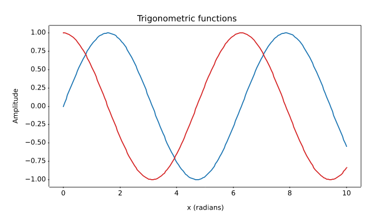
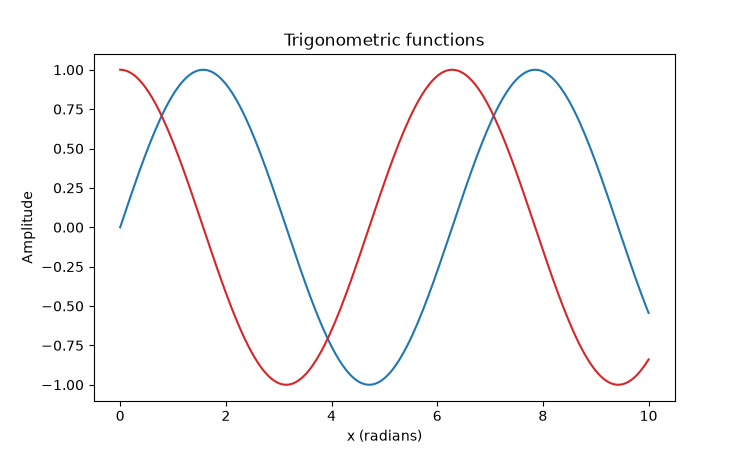
Two trigonometric series

PNG 10.5× faster
Matplotvite · 9.08 ms72.3 KiB
Matplotvite render of Two trigonometric series
matplotlib · Agg · 95.1 ms
matplotlib render of Two trigonometric series
Python source
import numpy as np
import matplotvite as plt

x = np.linspace(0, 10, 200)
plt.figure(figsize=(7.5, 4.5))
plt.plot(x, np.sin(x), label="sin(x)", color="#1f77b4")
plt.plot(x, np.cos(x), label="cos(x)", color="#d62728")
plt.title("Trigonometric functions")
plt.xlabel("x (radians)")
plt.ylabel("Amplitude")
plt.savefig("trigonometric_waves.png")
Line plots

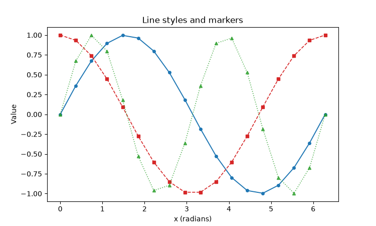
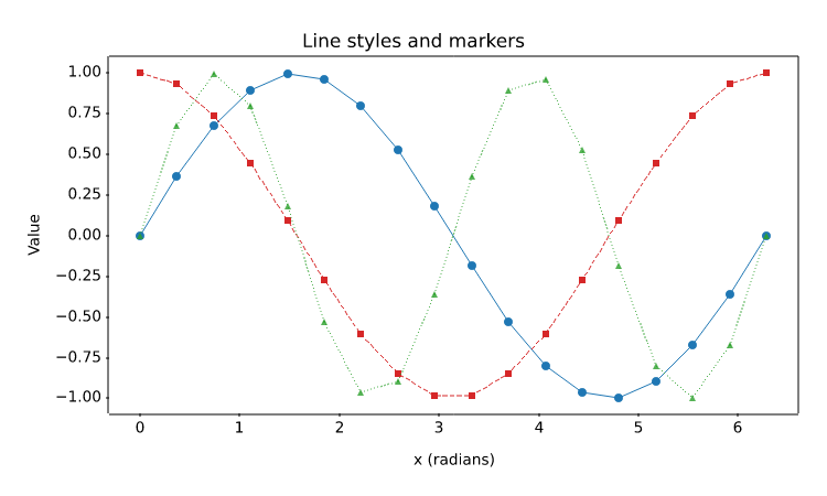
Line styles and markers

PNG 8.9× faster
Matplotvite · 11.1 ms58.5 KiB
Matplotvite render of Line styles and markers
matplotlib · Agg · 98.5 ms
matplotlib render of Line styles and markers
Python source
import numpy as np
import matplotvite as plt

x = np.linspace(0, 2 * np.pi, 18)
plt.figure(figsize=(7.5, 4.5))
plt.plot(x, np.sin(x), "o-", color="#1f77b4", linewidth=1.4,
         markersize=4, label="sin(x), solid")
plt.plot(x, np.cos(x), "s--", color="#d62728", linewidth=1.2,
         markersize=4, label="cos(x), dashed")
plt.plot(x, np.sin(2 * x), "^:", color="#2ca02c", linewidth=1.2,
         markersize=4, alpha=0.8, label="sin(2x), dotted")
plt.title("Line styles and markers")
plt.xlabel("x (radians)")
plt.ylabel("Value")
plt.savefig("line_styles_markers.png")
Line plots

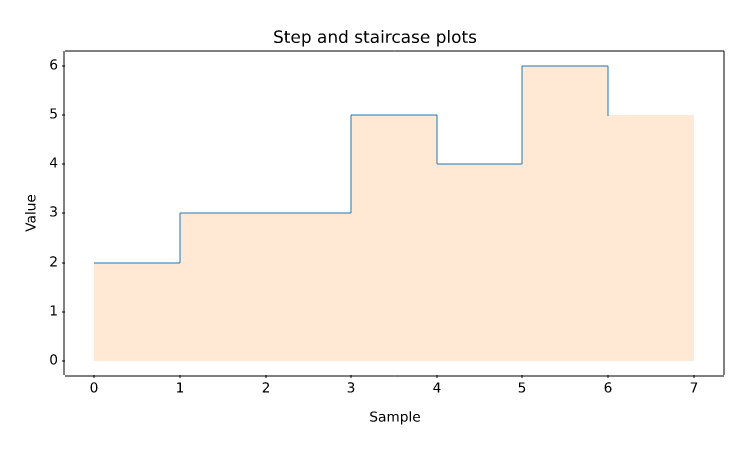
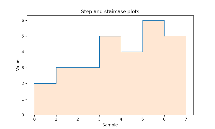
Step and staircase plots

PNG 8.3× faster
Matplotvite · 9.33 ms34.5 KiB
Matplotvite render of Step and staircase plots
matplotlib · Agg · 77.5 ms
matplotlib render of Step and staircase plots
Python source
import numpy as np
import matplotvite as plt

edges = np.arange(8, dtype=float)
y = np.array([2, 3, 3, 5, 4, 6, 5], dtype=float)
plt.figure(figsize=(7.5, 4.5))
plt.step(edges[:-1], y, where="post", color="#1f77b4", linewidth=1.4,
         label="step (post)")
plt.stairs(y, edges=edges, baseline=0, fill=True, alpha=0.18,
           color="#ff7f0e", label="stairs (filled)")
plt.title("Step and staircase plots")
plt.xlabel("Sample")
plt.ylabel("Value")
plt.savefig("step_stairs.png")
Line plots

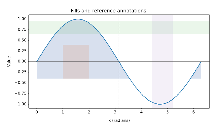
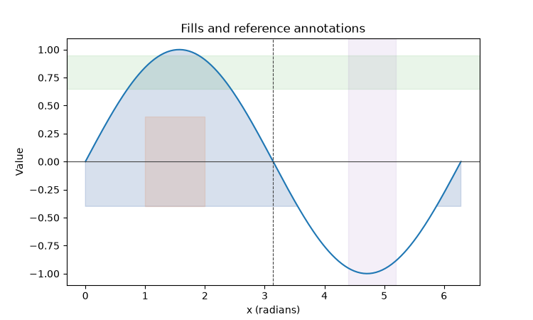
Fills, reference lines, and spans

PNG 9.6× faster
Matplotvite · 10.7 ms56.3 KiB
Matplotvite render of Fills, reference lines, and spans
matplotlib · Agg · 103.1 ms
matplotlib render of Fills, reference lines, and spans
Python source
import numpy as np
import matplotvite as plt

x = np.linspace(0, 2 * np.pi, 240)
y = np.sin(x)
plt.figure(figsize=(7.5, 4.5))
plt.plot(x, y, color="#1f77b4", linewidth=1.5, label="sin(x)")
plt.fill_between(x, y, -0.4, where=y > -0.4, color="#4c72b0",
                 alpha=0.22, label="y > -0.4")
plt.fill_betweenx(np.array([-0.4, 0.4]), 1.0, 2.0,
                  color="#dd8452", alpha=0.18)
plt.axhline(0, color="#444444", linewidth=0.8)
plt.axvline(np.pi, color="#444444", linewidth=0.8, linestyle="--")
plt.axhspan(0.65, 0.95, alpha=0.10, color="#2ca02c")
plt.axvspan(4.4, 5.2, alpha=0.10, color="#9467bd")
plt.title("Fills and reference annotations")
plt.xlabel("x (radians)")
plt.ylabel("Value")
plt.savefig("fill_regions.png")
Line plots

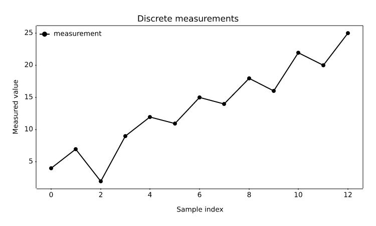
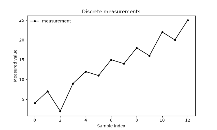
Implicit x indices

PNG 10.2× faster
Matplotvite · 8.27 ms48.5 KiB
Matplotvite render of Implicit x indices
matplotlib · Agg · 84.7 ms
matplotlib render of Implicit x indices
Python source
import matplotvite as plt

samples = [4, 7, 2, 9, 12, 11, 15, 14, 18, 16, 22, 20, 25]
plt.figure(figsize=(7.5, 4.5))
plt.plot(samples, label="measurement", color="black", marker="o",
         markersize=4)
plt.title("Discrete measurements")
plt.xlabel("Sample index")
plt.ylabel("Measured value")
plt.legend(frameon=False, loc="upper left")
plt.savefig("discrete_signal.png")
Line plots

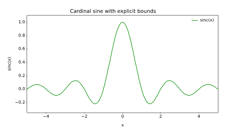
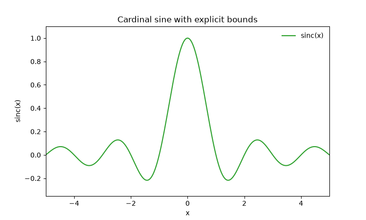
Explicit axis limits

PNG 10.0× faster
Matplotvite · 8.58 ms51.9 KiB
Matplotvite render of Explicit axis limits
matplotlib · Agg · 86.2 ms
matplotlib render of Explicit axis limits
Python source
import numpy as np
import matplotvite as plt

x = np.linspace(-6, 6, 300)
plt.figure(figsize=(7.5, 4.5))
plt.plot(x, np.sinc(x), label="sinc(x)", color="#2ca02c")
plt.xlim(-5.0, 5.0)
plt.ylim(-0.35, 1.1)
plt.title("Cardinal sine with explicit bounds")
plt.xlabel("x")
plt.ylabel("sinc(x)")
plt.legend(frameon=False, loc="upper right")
plt.savefig("custom_limits.png")
Statistical plots

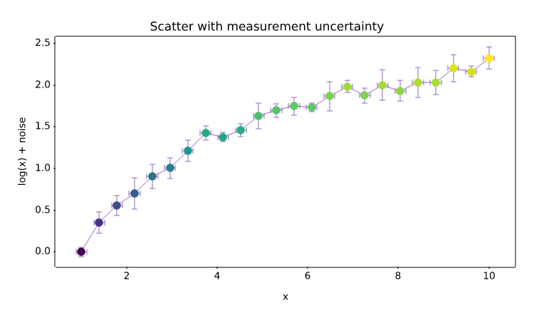
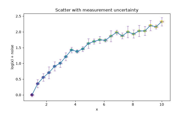
Scatter and error bars

PNG 9.8× faster
Matplotvite · 8.67 ms51.2 KiB
Matplotvite render of Scatter and error bars
matplotlib · Agg · 84.8 ms
matplotlib render of Scatter and error bars
Python source
import numpy as np
import matplotvite as plt

rng = np.random.default_rng(7)
x = np.linspace(1, 10, 24)
y = np.log(x) + rng.normal(0, 0.08, x.size)
yerr = rng.uniform(0.05, 0.2, x.size)
plt.figure(figsize=(7.5, 4.5))
plt.errorbar(x, y, yerr=yerr, xerr=0.12, fmt="", capsize=3,
             ecolor="#9467bd", elinewidth=0.9)
plt.scatter(x, y, s=48, c=y, cmap="viridis", marker="o")
plt.title("Scatter with measurement uncertainty")
plt.xlabel("x")
plt.ylabel("log(x) + noise")
plt.savefig("scatter_errorbar.png")
Statistical plots

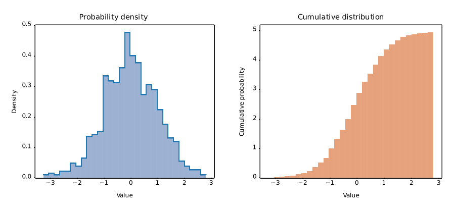
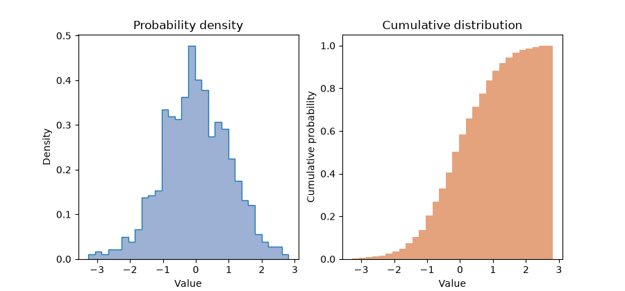
Histogram and cumulative density

PNG 23.3× faster
Matplotvite · 5.49 ms95.9 KiB
Matplotvite render of Histogram and cumulative density
matplotlib · Agg · 127.7 ms
matplotlib render of Histogram and cumulative density
Python source
import numpy as np
import matplotvite as plt

rng = np.random.default_rng(4)
data = rng.normal(loc=0.0, scale=1.0, size=900)
fig, axs = plt.subplots(1, 2, figsize=(9.0, 4.2))
axs[0].hist(data, bins=30, density=True, color="#4c72b0", alpha=0.55,
            label="density")
axs[0].hist(data, bins=30, histtype="step", density=True,
            color="#1f77b4", label="outline")
axs[0].set_title("Probability density")
axs[0].set_xlabel("Value")
axs[0].set_ylabel("Density")
axs[1].hist(data, bins=30, cumulative=True, density=True,
            color="#dd8452", alpha=0.75)
axs[1].set_title("Cumulative distribution")
axs[1].set_xlabel("Value")
axs[1].set_ylabel("Cumulative probability")
fig.savefig("histogram_density.png")
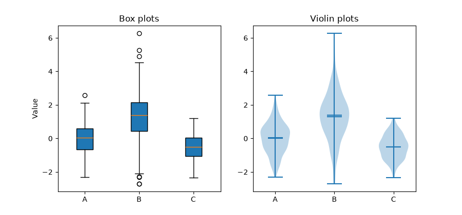
Statistical plots

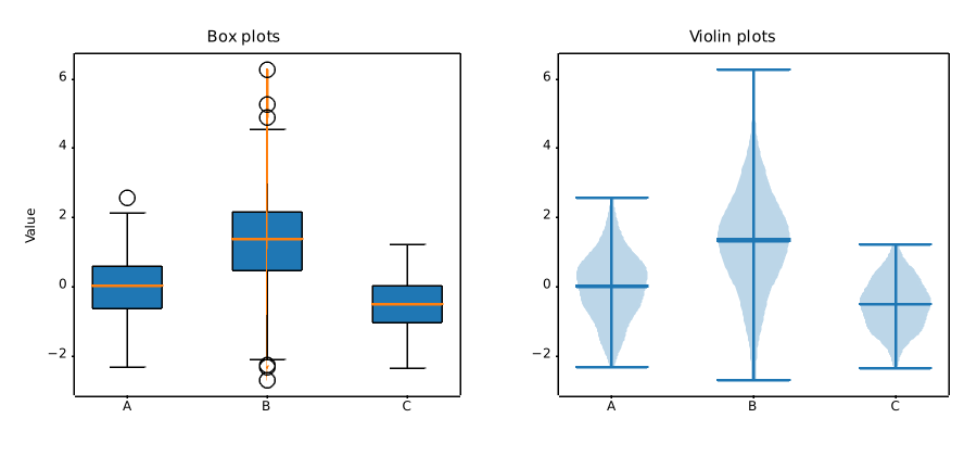
Box and violin summaries

PNG 12.2× faster
Matplotvite · 7.25 ms62.7 KiB
Matplotvite render of Box and violin summaries
matplotlib · Agg · 88.3 ms
matplotlib render of Box and violin summaries
Python source
import numpy as np
import matplotvite as plt

rng = np.random.default_rng(11)
groups = [
    rng.normal(0.0, 1.0, 240),
    rng.normal(1.2, 1.4, 240),
    rng.normal(-0.5, 0.7, 240),
]
labels = ["A", "B", "C"]
fig, axs = plt.subplots(1, 2, figsize=(9.0, 4.2))
axs[0].boxplot(groups, patch_artist=True, tick_labels=labels)
axs[0].set_title("Box plots")
axs[0].set_ylabel("Value")
axs[1].violinplot(groups, showmeans=True, showmedians=True)
axs[1].set_xticks([1, 2, 3], labels)
axs[1].set_title("Violin plots")
fig.savefig("box_violin.png")
Categorical data

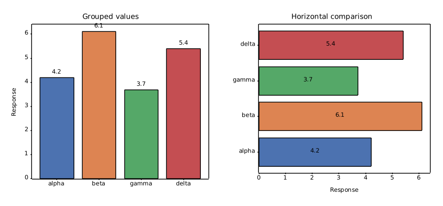
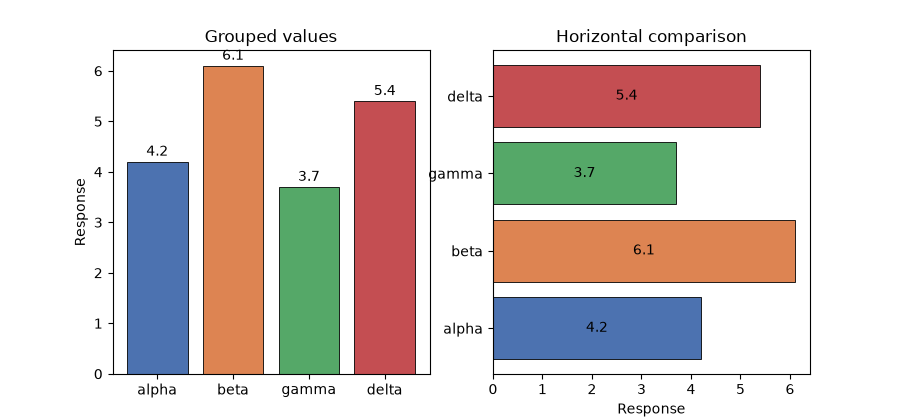
Vertical and horizontal bars

PNG 17.4× faster
Matplotvite · 5.22 ms80.2 KiB
Matplotvite render of Vertical and horizontal bars
matplotlib · Agg · 90.7 ms
matplotlib render of Vertical and horizontal bars
Python source
import numpy as np
import matplotvite as plt

labels = ["alpha", "beta", "gamma", "delta"]
values = np.array([4.2, 6.1, 3.7, 5.4])
colors = ["#4c72b0", "#dd8452", "#55a868", "#c44e52"]
positions = np.arange(len(labels))
fig, axs = plt.subplots(1, 2, figsize=(9.0, 4.2))
bars = axs[0].bar(positions, values, color=colors, edgecolor="black",
                  linewidth=0.6)
axs[0].bar_label(bars, fmt="%.1f", padding=2)
axs[0].set_xticks(positions, labels)
axs[0].set_ylabel("Response")
axs[0].set_title("Grouped values")
hbars = axs[1].barh(positions, values, color=colors, edgecolor="black",
                    linewidth=0.6)
axs[1].bar_label(hbars, fmt="%.1f", label_type="center")
axs[1].set_yticks(positions, labels)
axs[1].set_xlabel("Response")
axs[1].set_title("Horizontal comparison")
fig.savefig("bar_labels.png")
Categorical data

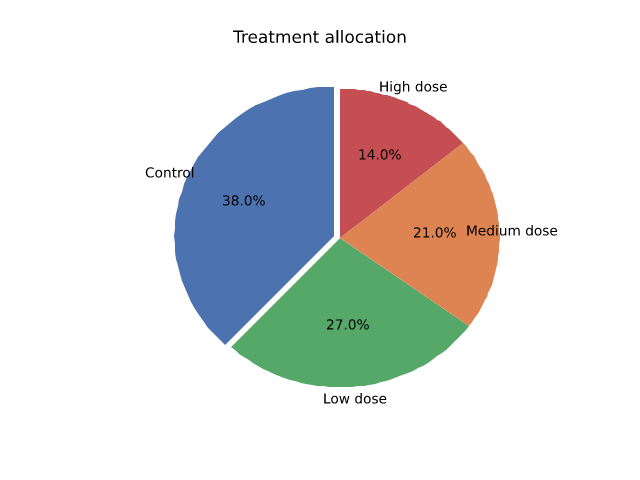
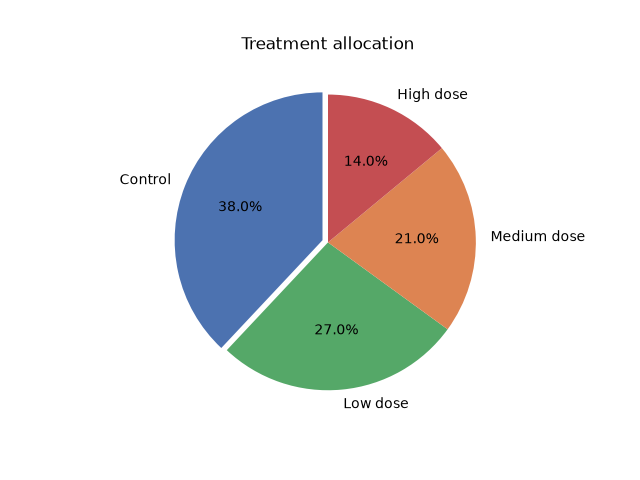
Part-to-whole composition

PNG 7.6× faster
Matplotvite · 6.39 ms38.1 KiB
Matplotvite render of Part-to-whole composition
matplotlib · Agg · 48.9 ms
matplotlib render of Part-to-whole composition
Python source
import matplotvite as plt

labels = ["Control", "Low dose", "Medium dose", "High dose"]
sizes = [38, 27, 21, 14]
colors = ["#4c72b0", "#55a868", "#dd8452", "#c44e52"]
plt.figure(figsize=(6.4, 4.8))
plt.pie(sizes, labels=labels, colors=colors, autopct="%1.1f%%",
        explode=(0.04, 0.0, 0.0, 0.0), startangle=90)
plt.title("Treatment allocation")
plt.savefig("pie_chart.png")
Categorical data

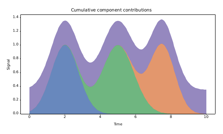
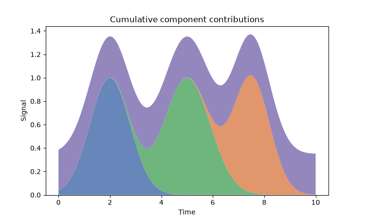
Cumulative area chart

PNG 11.1× faster
Matplotvite · 8.34 ms54.7 KiB
Matplotvite render of Cumulative area chart
matplotlib · Agg · 92.3 ms
matplotlib render of Cumulative area chart
Python source
import numpy as np
import matplotvite as plt

x = np.linspace(0, 10, 160)
components = [
    np.exp(-((x - 2.0) ** 2) / 1.2),
    np.exp(-((x - 5.0) ** 2) / 1.6),
    np.exp(-((x - 7.5) ** 2) / 1.0),
    0.35 * np.ones_like(x),
]
plt.figure(figsize=(7.5, 4.5))
plt.stackplot(x, *components, labels=["early", "middle", "late", "baseline"],
              colors=["#4c72b0", "#55a868", "#dd8452", "#8172b3"], alpha=0.85)
plt.title("Cumulative component contributions")
plt.xlabel("Time")
plt.ylabel("Signal")
plt.savefig("stackplot.png")
Statistical plots

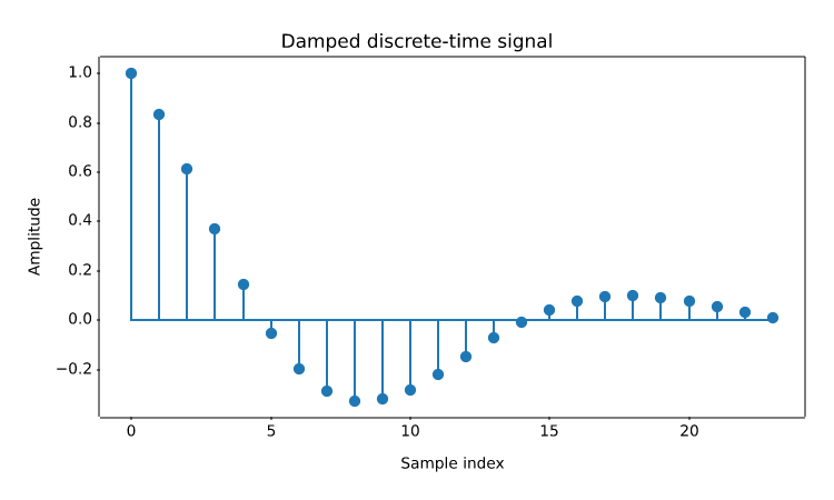
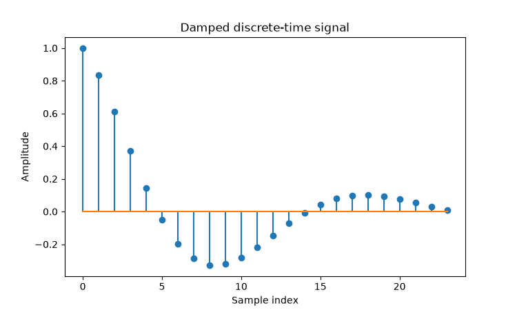
Stem plot

PNG 10.5× faster
Matplotvite · 7.77 ms51.6 KiB
Matplotvite render of Stem plot
matplotlib · Agg · 81.5 ms
matplotlib render of Stem plot
Python source
import numpy as np
import matplotvite as plt

n = np.arange(24)
y = np.exp(-n / 8.0) * np.cos(n / 3.0)
plt.figure(figsize=(7.5, 4.5))
plt.stem(n, y, linefmt="-", markerfmt="o", basefmt="-")
plt.title("Damped discrete-time signal")
plt.xlabel("Sample index")
plt.ylabel("Amplitude")
plt.savefig("stem_signal.png")
Statistical plots

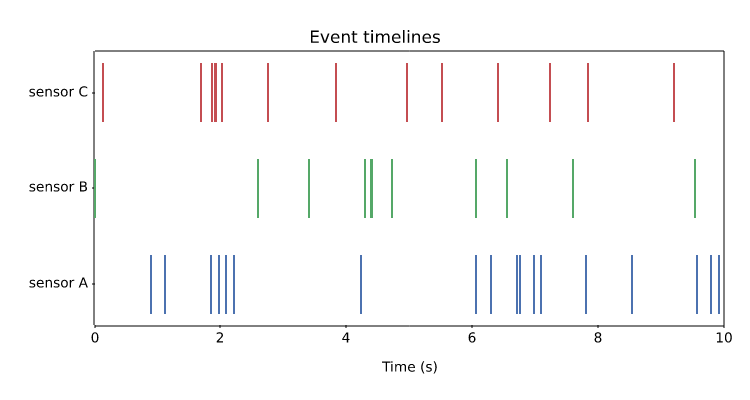
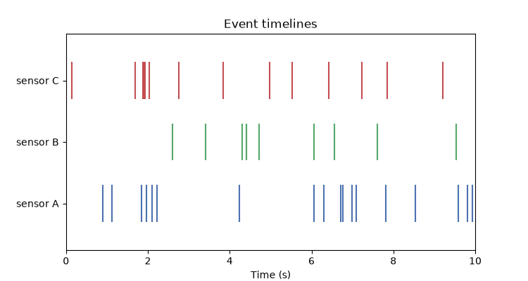
Event timelines

PNG 6.9× faster
Matplotvite · 8.30 ms53.5 KiB
Matplotvite render of Event timelines
matplotlib · Agg · 57.3 ms
matplotlib render of Event timelines
Python source
import numpy as np
import matplotvite as plt

rng = np.random.default_rng(21)
rows = [
    np.sort(rng.uniform(0, 10, 18)),
    np.sort(rng.uniform(0, 10, 11)),
    np.sort(rng.uniform(0, 10, 14)),
]
plt.figure(figsize=(7.5, 4.0))
plt.eventplot(rows, lineoffsets=[1.0, 2.0, 3.0],
              colors=["#4c72b0", "#55a868", "#c44e52"], linelengths=0.6)
plt.yticks([1, 2, 3], ["sensor A", "sensor B", "sensor C"])
plt.xlim(0, 10)
plt.xlabel("Time (s)")
plt.title("Event timelines")
plt.savefig("event_timeline.png")
Statistical plots

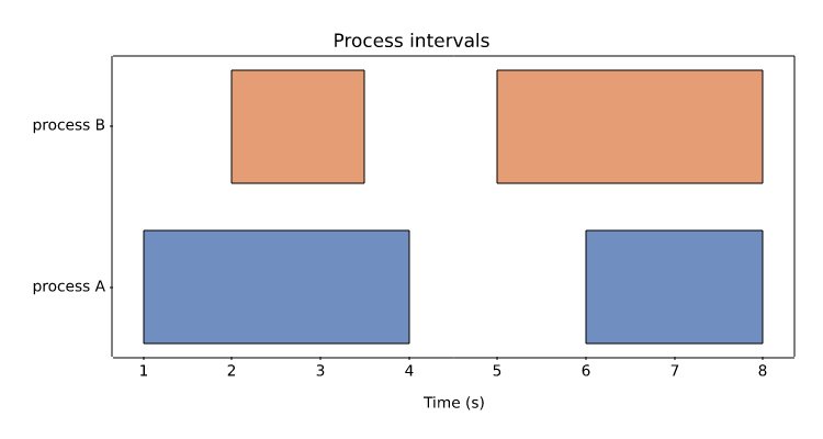
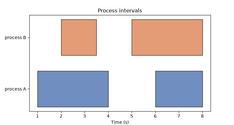
Broken horizontal bars

PNG 9.2× faster
Matplotvite · 6.47 ms37.7 KiB
Matplotvite render of Broken horizontal bars
matplotlib · Agg · 59.9 ms
matplotlib render of Broken horizontal bars
Python source
import matplotvite as plt

plt.figure(figsize=(7.5, 4.0))
plt.broken_barh([(1, 3), (6, 2)], (2, 0.7), facecolors="#4c72b0",
                edgecolor="black", alpha=0.8)
plt.broken_barh([(2, 1.5), (5, 3)], (3, 0.7), facecolors="#dd8452",
                edgecolor="black", alpha=0.8)
plt.yticks([2.35, 3.35], ["process A", "process B"])
plt.xlabel("Time (s)")
plt.title("Process intervals")
plt.savefig("broken_barh.png")
Gridded data

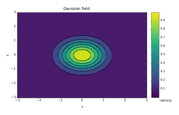
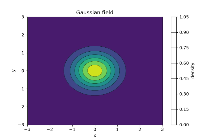
Filled and line contours

PNG 14.5× faster
Matplotvite · 8.29 ms60.5 KiB
Matplotvite render of Filled and line contours
matplotlib · Agg · 120.4 ms
matplotlib render of Filled and line contours
Python source
import numpy as np
import matplotvite as plt

x = np.linspace(-3, 3, 120)
y = np.linspace(-3, 3, 120)
z = np.exp(-(x[None, :] ** 2 + y[:, None] ** 2))
plt.figure(figsize=(7.0, 4.5))
plt.contourf(x, y, z, levels=8, cmap="viridis")
plt.contour(x, y, z, levels=8, colors="black", linewidths=0.4)
plt.colorbar(label="density")
plt.title("Gaussian field")
plt.xlabel("x")
plt.ylabel("y")
plt.savefig("contours_colorbar.png")
Gridded data

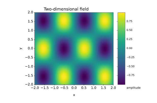
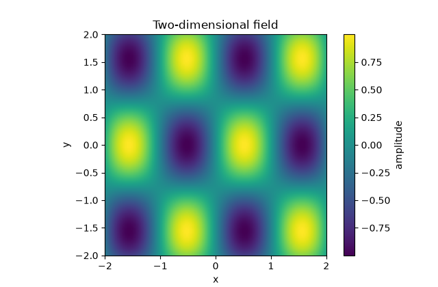
Image heatmap

PNG 16.2× faster
Matplotvite · 9.57 ms172.9 KiB
Matplotvite render of Image heatmap
matplotlib · Agg · 155.0 ms
matplotlib render of Image heatmap
Python source
import numpy as np
import matplotvite as plt

x = np.linspace(-2, 2, 240)
y = np.linspace(-2, 2, 140)
z = np.sin(3 * x[None, :]) * np.cos(2 * y[:, None])
plt.figure(figsize=(6.4, 4.2))
plt.imshow(z, cmap="viridis", extent=(-2, 2, -2, 2), origin="lower")
plt.colorbar(label="amplitude")
plt.title("Two-dimensional field")
plt.xlabel("x")
plt.ylabel("y")
plt.savefig("imshow_heatmap.png")
Gridded data

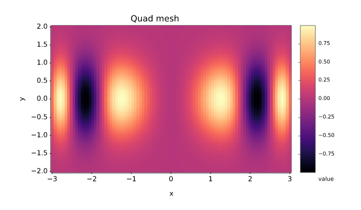
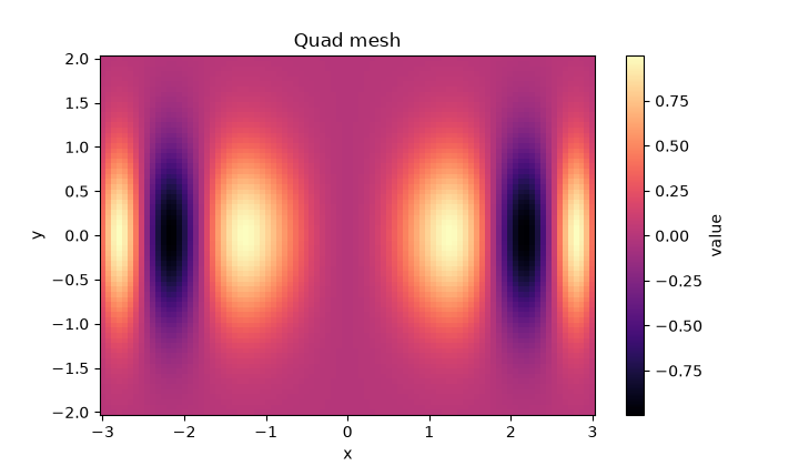
Quad mesh

PNG 14.2× faster
Matplotvite · 9.12 ms122.2 KiB
Matplotvite render of Quad mesh
matplotlib · Agg · 129.9 ms
matplotlib render of Quad mesh
Python source
import numpy as np
import matplotvite as plt

x = np.linspace(-3, 3, 90)
y = np.linspace(-2, 2, 70)
z = np.sin(x[None, :] ** 2) * np.exp(-y[:, None] ** 2)
plt.figure(figsize=(7.2, 4.2))
plt.pcolormesh(x, y, z, cmap="magma", shading="auto")
plt.colorbar(label="value")
plt.title("Quad mesh")
plt.xlabel("x")
plt.ylabel("y")
plt.savefig("pcolormesh.png")
Gridded data

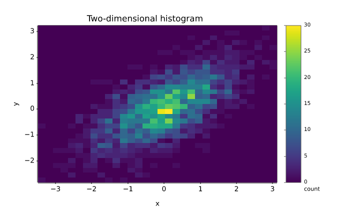
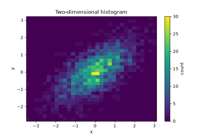
Bivariate density

PNG 8.4× faster
Matplotvite · 8.84 ms56.7 KiB
Matplotvite render of Bivariate density
matplotlib · Agg · 74.0 ms
matplotlib render of Bivariate density
Python source
import numpy as np
import matplotvite as plt

rng = np.random.default_rng(5)
x = rng.normal(0, 1, 2400)
y = 0.6 * x + rng.normal(0, 0.7, x.size)
fig, ax = plt.subplots(figsize=(6.8, 4.4))
hist = ax.hist2d(x, y, bins=32, cmap="viridis")
fig.colorbar(hist[3], label="count")
ax.set_title("Two-dimensional histogram")
ax.set_xlabel("x")
ax.set_ylabel("y")
fig.savefig("hist2d_hexbin.png")
Gridded data

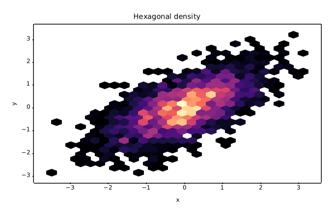
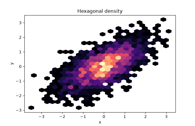
Hexagonal binning

PNG 8.7× faster
Matplotvite · 6.51 ms68.4 KiB
Matplotvite render of Hexagonal binning
matplotlib · Agg · 56.9 ms
matplotlib render of Hexagonal binning
Python source
import numpy as np
import matplotvite as plt

rng = np.random.default_rng(5)
x = rng.normal(0, 1, 2400)
y = 0.6 * x + rng.normal(0, 0.7, x.size)
fig, ax = plt.subplots(figsize=(6.8, 4.4))
ax.hexbin(x, y, gridsize=26, cmap="magma", mincnt=1)
ax.set_title("Hexagonal density")
ax.set_xlabel("x")
ax.set_ylabel("y")
fig.savefig("hexbin_density.png")
Gridded data

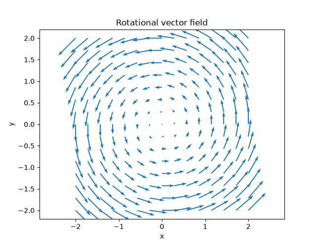
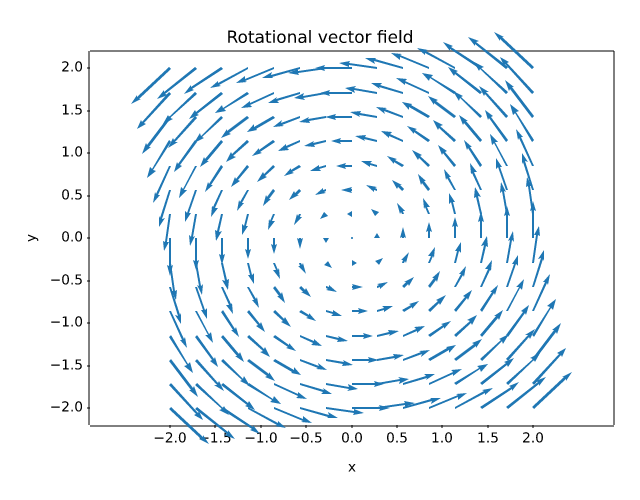
Vector field

PNG 9.6× faster
Matplotvite · 9.45 ms135.3 KiB
Matplotvite render of Vector field
matplotlib · Agg · 90.3 ms
matplotlib render of Vector field
Python source
import numpy as np
import matplotvite as plt

x = np.linspace(-2, 2, 15)
y = np.linspace(-2, 2, 15)
X, Y = np.meshgrid(x, y)
U, V = -Y, X
plt.figure(figsize=(6.4, 5.0))
plt.quiver(X, Y, U, V, color="#1f77b4", scale=28)
plt.axis("equal")
plt.title("Rotational vector field")
plt.xlabel("x")
plt.ylabel("y")
plt.savefig("quiver_field.png")
Annotations and axes

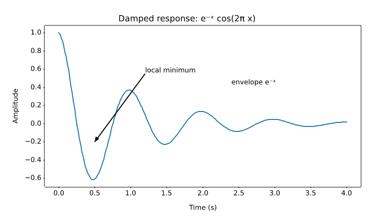
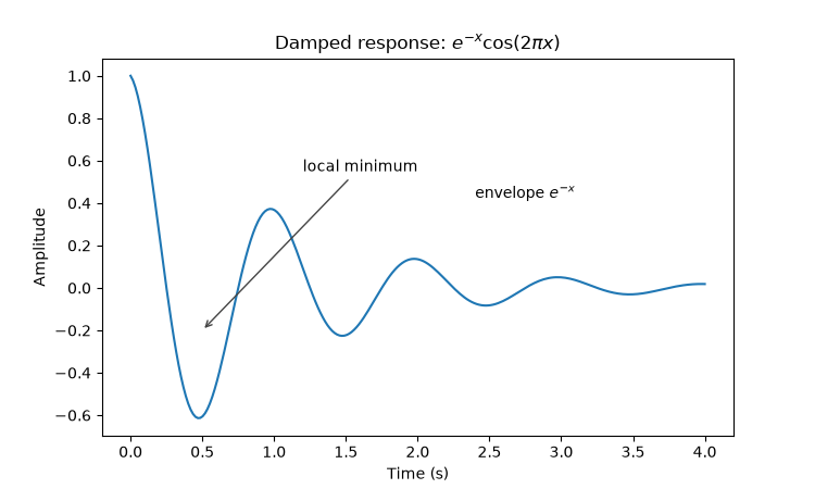
Annotations and mathematics

PNG 15.8× faster
Matplotvite · 7.70 ms60.0 KiB
Matplotvite render of Annotations and mathematics
matplotlib · Agg · 122.0 ms
matplotlib render of Annotations and mathematics
Python source
import numpy as np
import matplotvite as plt

x = np.linspace(0, 4, 240)
y = np.exp(-x) * np.cos(2 * np.pi * x)
plt.figure(figsize=(7.5, 4.5))
plt.plot(x, y, color="#1f77b4", linewidth=1.5)
plt.annotate("local minimum", xy=(0.5, -0.20), xytext=(1.2, 0.55),
             arrowprops=dict(arrowstyle="->", color="#444444"))
plt.text(2.4, 0.42, r"envelope $e^{-x}$", fontsize=10)
plt.title(r"Damped response: $e^{-x} \cos(2\pi x)$")
plt.xlabel("Time (s)")
plt.ylabel("Amplitude")
plt.savefig("annotations_mathtext.png")
Annotations and axes

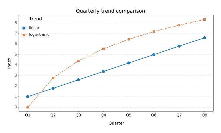
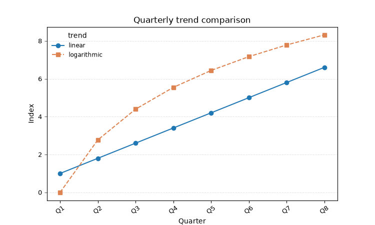
Ticks, grid, and legend layout

PNG 7.2× faster
Matplotvite · 12.9 ms69.3 KiB
Matplotvite render of Ticks, grid, and legend layout
matplotlib · Agg · 92.9 ms
matplotlib render of Ticks, grid, and legend layout
Python source
import numpy as np
import matplotvite as plt

x = np.arange(8)
plt.figure(figsize=(7.5, 4.5))
plt.plot(x, 0.8 * x + 1.0, "o-", label="linear", color="#1f77b4")
plt.plot(x, 4.0 * np.log1p(x), "s--", label="logarithmic",
         color="#dd8452")
plt.xticks(x, ["Q1", "Q2", "Q3", "Q4", "Q5", "Q6", "Q7", "Q8"],
           rotation=35, fontsize=9)
plt.tick_params(axis="y", labelsize=9, color="#666666")
plt.grid(True, axis="y", linestyle="--", linewidth=0.7, alpha=0.35)
plt.legend(title="trend", loc="upper left", frameon=False, fontsize=8.5)
plt.title("Quarterly trend comparison")
plt.xlabel("Quarter")
plt.ylabel("Index")
plt.savefig("ticks_grid_legend.png")
Annotations and axes

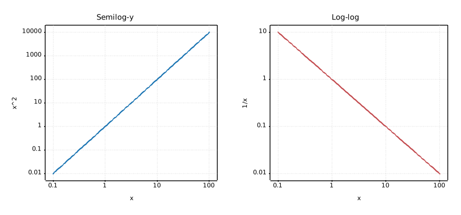
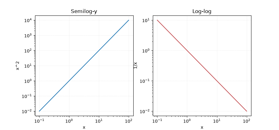
Logarithmic scales

PNG 57.9× faster
Matplotvite · 4.24 ms83.5 KiB
Matplotvite render of Logarithmic scales
matplotlib · Agg · 245.6 ms
matplotlib render of Logarithmic scales
Python source
import numpy as np
import matplotvite as plt

x = np.logspace(-1, 2, 120)
fig, axs = plt.subplots(1, 2, figsize=(9.0, 4.2))
axs[0].semilogy(x, x ** 2, color="#1f77b4", label="x^2")
axs[0].set_xscale("log")
axs[0].set_title("Semilog-y")
axs[0].set_xlabel("x")
axs[0].set_ylabel("x^2")
axs[1].loglog(x, 1.0 / x, color="#c44e52", label="1/x")
axs[1].set_title("Log-log")
axs[1].set_xlabel("x")
axs[1].set_ylabel("1/x")
for ax in axs:
    ax.grid(True, which="major", linestyle=":", alpha=0.35)
fig.savefig("log_scales.png")
Layout

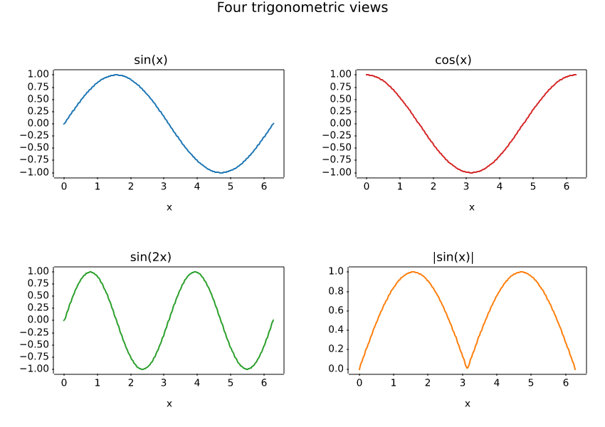
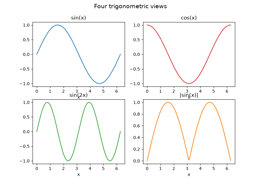
2x2 subplot grid

PNG 11.2× faster
Matplotvite · 14.2 ms109.0 KiB
Matplotvite render of 2x2 subplot grid
matplotlib · Agg · 159.6 ms
matplotlib render of 2x2 subplot grid
Python source
import numpy as np
import matplotvite as plt

x = np.linspace(0, 2 * np.pi, 220)
fig, axs = plt.subplots(2, 2, figsize=(8.5, 6.0))
axs[0, 0].plot(x, np.sin(x), color="#1f77b4")
axs[0, 0].set_title("sin(x)")
axs[0, 1].plot(x, np.cos(x), color="#d62728")
axs[0, 1].set_title("cos(x)")
axs[1, 0].plot(x, np.sin(2 * x), color="#2ca02c")
axs[1, 0].set_title("sin(2x)")
axs[1, 1].plot(x, np.abs(np.sin(x)), color="#ff7f0e")
axs[1, 1].set_title("|sin(x)|")
for ax in axs.flat:
    ax.set_xlabel("x")
fig.suptitle("Four trigonometric views", fontsize=14)
fig.savefig("subplots_grid.png")
Layout

Stateful subplot API

PNG 31.3× faster
Matplotvite · 4.31 ms62.0 KiB
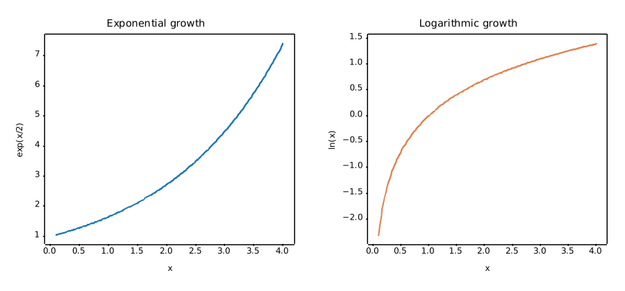
Matplotvite render of Stateful subplot API
matplotlib · Agg · 135.0 ms
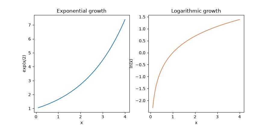
matplotlib render of Stateful subplot API
Python source
import numpy as np
import matplotvite as plt

x = np.linspace(0.1, 4.0, 180)
plt.figure(figsize=(9.0, 4.2))
plt.subplot(1, 2, 1)
plt.plot(x, np.exp(x / 2), color="#1f77b4", label="exp(x/2)")
plt.title("Exponential growth")
plt.xlabel("x")
plt.ylabel("exp(x/2)")
plt.subplot(1, 2, 2)
plt.plot(x, np.log(x), color="#dd8452", label="ln(x)")
plt.title("Logarithmic growth")
plt.xlabel("x")
plt.ylabel("ln(x)")
plt.savefig("side_by_side.png")
Layout

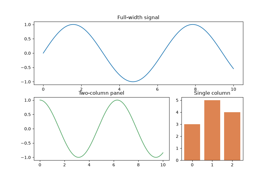
GridSpec spans

PNG 9.8× faster
Matplotvite · 11.8 ms89.3 KiB
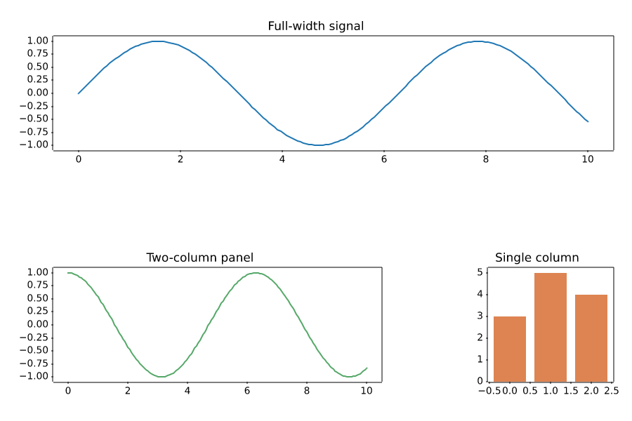
Matplotvite render of GridSpec spans
matplotlib · Agg · 115.7 ms
matplotlib render of GridSpec spans
Python source
import numpy as np
import matplotvite as plt

fig = plt.figure(figsize=(9.0, 6.0))
gs = fig.add_gridspec(2, 3)
top = fig.add_subplot(gs[0, :])
left = fig.add_subplot(gs[1, 0:2])
right = fig.add_subplot(gs[1, 2])
x = np.linspace(0, 10, 180)
top.plot(x, np.sin(x), color="#1f77b4")
top.set_title("Full-width signal")
left.plot(x, np.cos(x), color="#55a868")
left.set_title("Two-column panel")
right.bar([0, 1, 2], [3, 5, 4], color="#dd8452")
right.set_title("Single column")
fig.savefig("gridspec_layout.png")
Layout

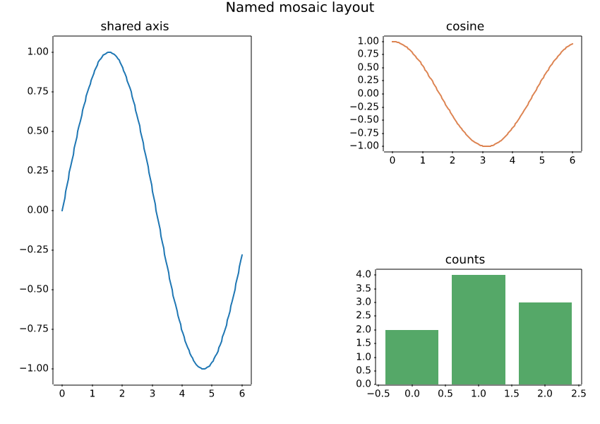
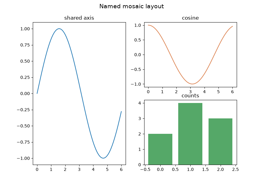
Mosaic layout

PNG 11.4× faster
Matplotvite · 11.8 ms100.1 KiB
Matplotvite render of Mosaic layout
matplotlib · Agg · 133.9 ms
matplotlib render of Mosaic layout
Python source
import numpy as np
import matplotvite as plt

fig, axes = plt.subplot_mosaic(
    [["left", "right"], ["left", "bottom"]], figsize=(8.5, 6.0)
)
x = np.linspace(0, 6, 150)
axes["left"].plot(x, np.sin(x), color="#1f77b4")
axes["left"].set_title("shared axis")
axes["right"].plot(x, np.cos(x), color="#dd8452")
axes["right"].set_title("cosine")
axes["bottom"].bar([0, 1, 2], [2, 4, 3], color="#55a868")
axes["bottom"].set_title("counts")
fig.suptitle("Named mosaic layout", fontsize=14)
fig.savefig("mosaic_layout.png")
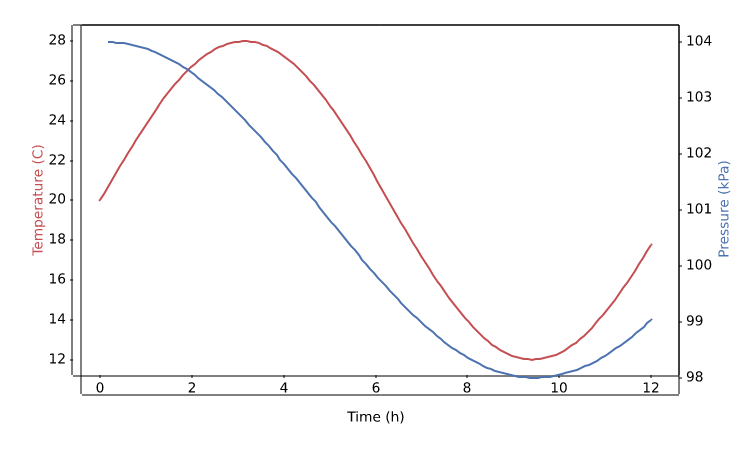
Layout

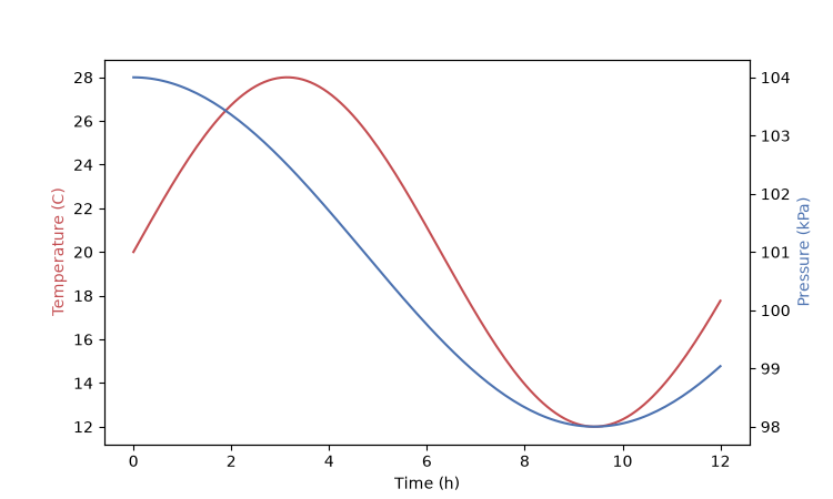
Twin axes

PNG 6.7× faster
Matplotvite · 11.6 ms62.6 KiB
Matplotvite render of Twin axes
matplotlib · Agg · 77.1 ms
matplotlib render of Twin axes
Python source
import numpy as np
import matplotvite as plt

x = np.linspace(0, 12, 140)
temperature = 20 + 8 * np.sin(x / 2.0)
pressure = 101 + 3 * np.cos(x / 3.0)
fig, ax_left = plt.subplots(figsize=(7.5, 4.5))
ax_left.plot(x, temperature, color="#c44e52", label="temperature")
ax_left.set_xlabel("Time (h)")
ax_left.set_ylabel("Temperature (C)", color="#c44e52")
ax_right = ax_left.twinx()
ax_right.plot(x, pressure, color="#4c72b0", label="pressure")
ax_right.set_ylabel("Pressure (kPa)", color="#4c72b0")
fig.savefig("twin_axes.png")
Data types

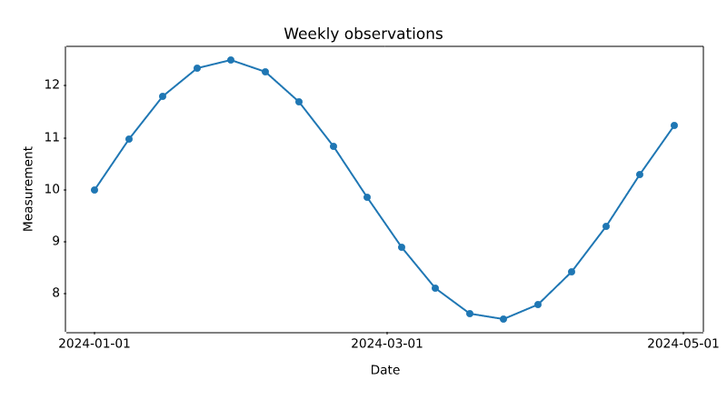
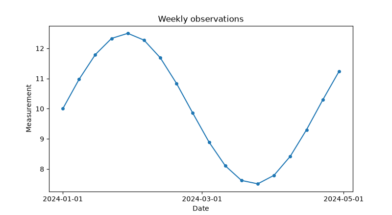
Date and time axis

PNG 10.2× faster
Matplotvite · 6.94 ms48.2 KiB
Matplotvite render of Date and time axis
matplotlib · Agg · 70.8 ms
matplotlib render of Date and time axis
Python source
from datetime import datetime, timedelta

import numpy as np
import matplotvite as plt

start = datetime(2024, 1, 1)
dates = [start + timedelta(days=7 * i) for i in range(18)]
values = 10 + 2.5 * np.sin(np.arange(len(dates)) / 2.5)
plt.figure(figsize=(8.0, 4.4))
plt.plot(dates, values, "o-", color="#1f77b4", markersize=4)
plt.xticks([datetime(2024, 1, 1), datetime(2024, 3, 1),
            datetime(2024, 5, 1)])
plt.title("Weekly observations")
plt.xlabel("Date")
plt.ylabel("Measurement")
plt.savefig("datetime_axis.png")
Data types

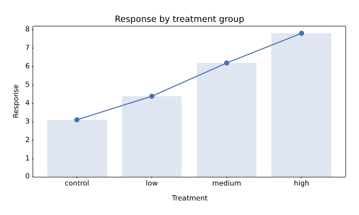
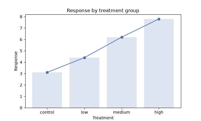
Categorical axis

PNG 11.4× faster
Matplotvite · 7.14 ms46.3 KiB
Matplotvite render of Categorical axis
matplotlib · Agg · 81.6 ms
matplotlib render of Categorical axis
Python source
import numpy as np
import matplotvite as plt

categories = ["control", "low", "medium", "high"]
values = np.array([3.1, 4.4, 6.2, 7.8])
plt.figure(figsize=(7.0, 4.2))
plt.plot(categories, values, "o-", color="#4c72b0", markersize=6)
plt.bar(categories, values, color="#4c72b0", alpha=0.18)
plt.title("Response by treatment group")
plt.xlabel("Treatment")
plt.ylabel("Response")
plt.savefig("categorical_axis.png")
Data types

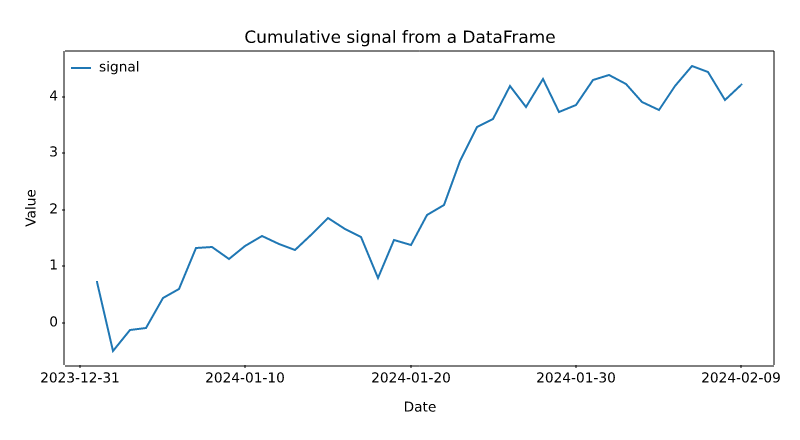
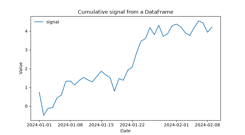
DataFrame columns

PNG 11.9× faster
Matplotvite · 7.98 ms56.3 KiB
Matplotvite render of DataFrame columns
matplotlib · Agg · 94.6 ms
matplotlib render of DataFrame columns
Python source
import numpy as np
import pandas as pd
import matplotvite as plt

rng = np.random.default_rng(13)
dates = pd.date_range("2024-01-01", periods=40, freq="D")
frame = pd.DataFrame(
    {"signal": np.cumsum(rng.normal(0, 0.4, dates.size))},
    index=dates,
)
plt.figure(figsize=(8.0, 4.4))
plt.plot("signal", data=frame, label="signal", color="#1f77b4")
plt.title("Cumulative signal from a DataFrame")
plt.xlabel("Date")
plt.ylabel("Value")
plt.legend(frameon=False, loc="upper left")
plt.savefig("pandas_frame.png")
Colormaps and styling

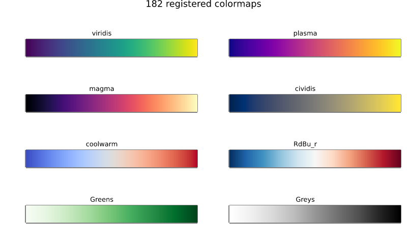
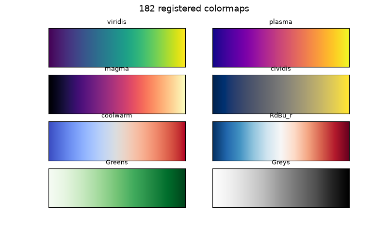
Colormap registry

PNG 8.0× faster
Matplotvite · 10.9 ms145.4 KiB
Matplotvite render of Colormap registry
matplotlib · Agg · 87.4 ms
matplotlib render of Colormap registry
Python source
import numpy as np
import matplotvite as plt

names = ["viridis", "plasma", "magma", "cividis",
         "coolwarm", "RdBu_r", "Greens", "Greys"]
gradient = np.linspace(0, 1, 256)[None, :]
fig, axs = plt.subplots(4, 2, figsize=(8.0, 4.8))
for ax, name in zip(axs.flat, names):
    ax.imshow(gradient, cmap=name, aspect="auto")
    ax.set_title(name, fontsize=9)
    ax.set_xticks([])
    ax.set_yticks([])
fig.suptitle(f"{len(plt.colormaps())} registered colormaps", fontsize=13)
fig.savefig("colormap_reference.png")
Colormaps and styling

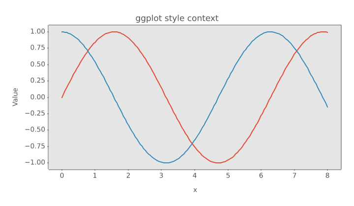
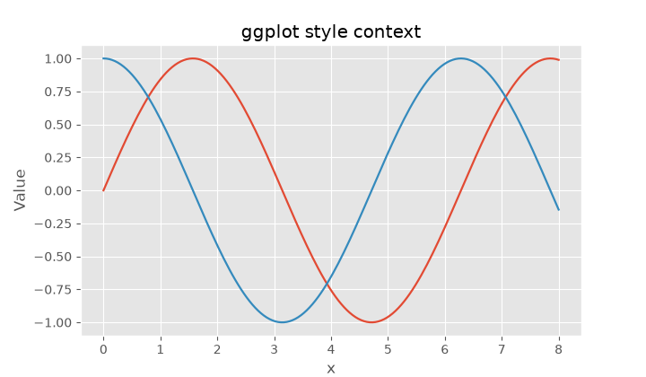
Style context

PNG 9.9× faster
Matplotvite · 6.94 ms56.3 KiB
Matplotvite render of Style context
matplotlib · Agg · 68.5 ms
matplotlib render of Style context
Python source
import numpy as np
import matplotvite as plt

x = np.linspace(0, 8, 160)
with plt.style.context("ggplot"):
    fig, ax = plt.subplots(figsize=(7.2, 4.2))
    ax.plot(x, np.sin(x), label="sin(x)", linewidth=1.6)
    ax.plot(x, np.cos(x), label="cos(x)", linewidth=1.6)
    ax.set_title("ggplot style context")
    ax.set_xlabel("x")
    ax.set_ylabel("Value")
    fig.savefig("style_context.png")
Output

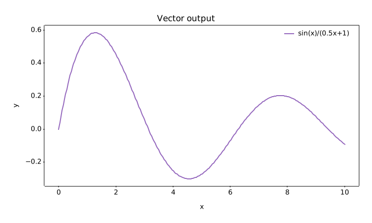
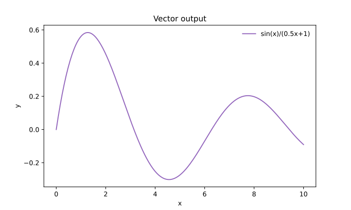
SVG output

SVG 87.5× faster
Matplotvite · 0.76 ms8.1 KiB
Matplotvite render of SVG output
matplotlib · Agg · 66.5 ms
matplotlib render of SVG output
Python source
import numpy as np
import matplotvite as plt

x = np.linspace(0, 10, 250)
y = np.sin(x) / (0.5 * x + 1.0)
plt.figure(figsize=(7.5, 4.5))
plt.plot(x, y, label="sin(x)/(0.5x+1)", color="#9467bd")
plt.title("Vector output")
plt.xlabel("x")
plt.ylabel("y")
plt.legend(frameon=False, loc="upper right")
plt.savefig("svg_export.svg")
Output

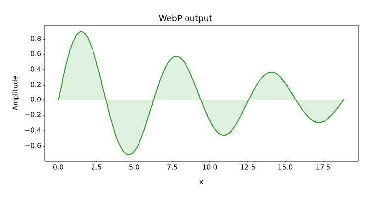
WebP output

WEBP
Matplotvite · 20.6 ms5.8 KiB
Matplotvite render of WebP output
matplotlib · skipped

This snippet uses an output format or dependency that the comparison build could not render with matplotlib.

Python source
import numpy as np
import matplotvite as plt

x = np.linspace(0, 6 * np.pi, 400)
plt.figure(figsize=(7.5, 4.0))
plt.plot(x, np.sin(x) * np.exp(-x / 14), color="#2ca02c")
plt.fill_between(x, np.sin(x) * np.exp(-x / 14), 0,
                 color="#2ca02c", alpha=0.15)
plt.title("WebP output")
plt.xlabel("x")
plt.ylabel("Amplitude")
plt.savefig("webp_export.webp")