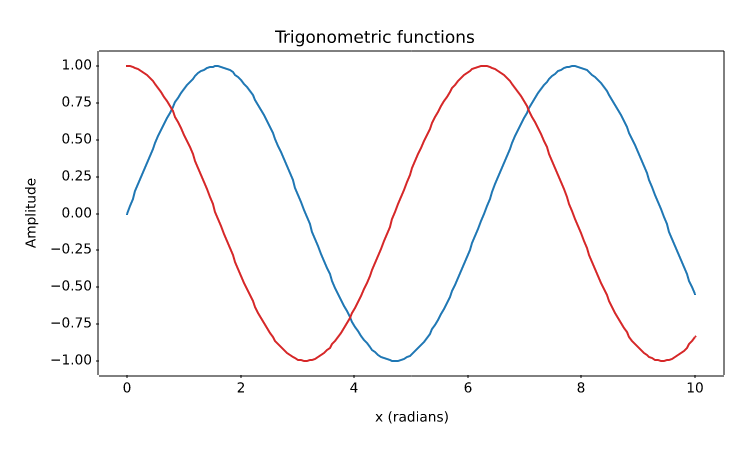
Two line series with explicit colours, a legend, and labelled axes.
import numpy as np
import matplotvite as plt

x = np.linspace(0, 10, 200)
plt.figure(figsize=(7.5, 4.5))
plt.plot(x, np.sin(x), label="sin(x)", color="#1f77b4")
plt.plot(x, np.cos(x), label="cos(x)", color="#d62728")
plt.title("Trigonometric functions")
plt.xlabel("x (radians)")
plt.ylabel("Amplitude")
plt.savefig("trigonometric_waves.png")
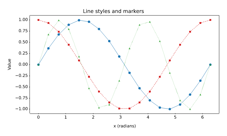
Format strings, dashed and dotted styles, line widths, markers, and alpha transparency.
import numpy as np
import matplotvite as plt

x = np.linspace(0, 2 * np.pi, 18)
plt.figure(figsize=(7.5, 4.5))
plt.plot(x, np.sin(x), "o-", color="#1f77b4", linewidth=1.4,
         markersize=4, label="sin(x), solid")
plt.plot(x, np.cos(x), "s--", color="#d62728", linewidth=1.2,
         markersize=4, label="cos(x), dashed")
plt.plot(x, np.sin(2 * x), "^:", color="#2ca02c", linewidth=1.2,
         markersize=4, alpha=0.8, label="sin(2x), dotted")
plt.title("Line styles and markers")
plt.xlabel("x (radians)")
plt.ylabel("Value")
plt.savefig("line_styles_markers.png")
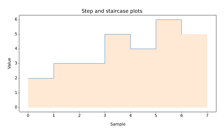
Piecewise-constant series drawn with step(), including a filled stairs() outline.
import numpy as np
import matplotvite as plt

edges = np.arange(8, dtype=float)
y = np.array([2, 3, 3, 5, 4, 6, 5], dtype=float)
plt.figure(figsize=(7.5, 4.5))
plt.step(edges[:-1], y, where="post", color="#1f77b4", linewidth=1.4,
         label="step (post)")
plt.stairs(y, edges=edges, baseline=0, fill=True, alpha=0.18,
           color="#ff7f0e", label="stairs (filled)")
plt.title("Step and staircase plots")
plt.xlabel("Sample")
plt.ylabel("Value")
plt.savefig("step_stairs.png")
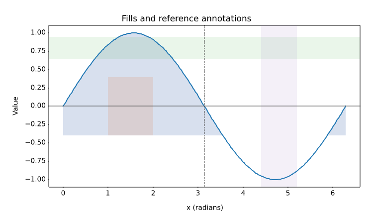
fill_between(), fill_betweenx(), axhline(), axvline(), and shaded axis spans.
import numpy as np
import matplotvite as plt

x = np.linspace(0, 2 * np.pi, 240)
y = np.sin(x)
plt.figure(figsize=(7.5, 4.5))
plt.plot(x, y, color="#1f77b4", linewidth=1.5, label="sin(x)")
plt.fill_between(x, y, -0.4, where=y > -0.4, color="#4c72b0",
                 alpha=0.22, label="y > -0.4")
plt.fill_betweenx(np.array([-0.4, 0.4]), 1.0, 2.0,
                  color="#dd8452", alpha=0.18)
plt.axhline(0, color="#444444", linewidth=0.8)
plt.axvline(np.pi, color="#444444", linewidth=0.8, linestyle="--")
plt.axhspan(0.65, 0.95, alpha=0.10, color="#2ca02c")
plt.axvspan(4.4, 5.2, alpha=0.10, color="#9467bd")
plt.title("Fills and reference annotations")
plt.xlabel("x (radians)")
plt.ylabel("Value")
plt.savefig("fill_regions.png")
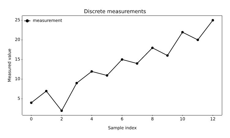
A one-dimensional sequence plotted against its implicit 0..N-1 index.
import matplotvite as plt

samples = [4, 7, 2, 9, 12, 11, 15, 14, 18, 16, 22, 20, 25]
plt.figure(figsize=(7.5, 4.5))
plt.plot(samples, label="measurement", color="black", marker="o",
         markersize=4)
plt.title("Discrete measurements")
plt.xlabel("Sample index")
plt.ylabel("Measured value")
plt.legend(frameon=False, loc="upper left")
plt.savefig("discrete_signal.png")
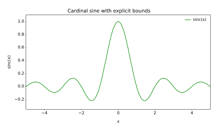
Zooming into a region of interest with xlim() and ylim().
import numpy as np
import matplotvite as plt

x = np.linspace(-6, 6, 300)
plt.figure(figsize=(7.5, 4.5))
plt.plot(x, np.sinc(x), label="sinc(x)", color="#2ca02c")
plt.xlim(-5.0, 5.0)
plt.ylim(-0.35, 1.1)
plt.title("Cardinal sine with explicit bounds")
plt.xlabel("x")
plt.ylabel("sinc(x)")
plt.legend(frameon=False, loc="upper right")
plt.savefig("custom_limits.png")
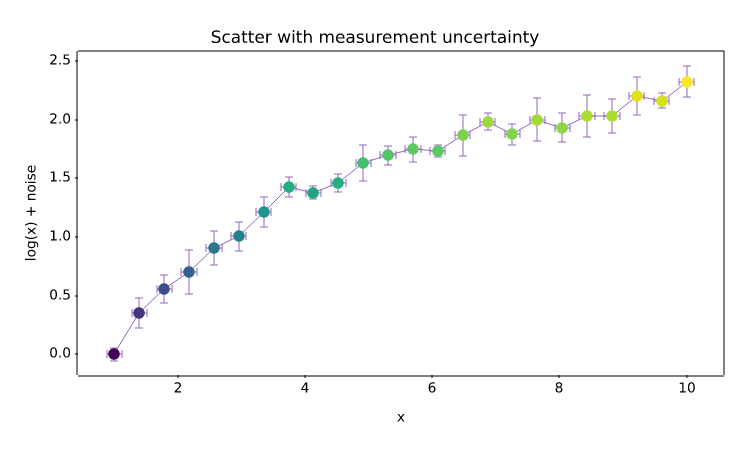
Per-point marker colours from a colormap, overlaid with x and y error bars.
import numpy as np
import matplotvite as plt

rng = np.random.default_rng(7)
x = np.linspace(1, 10, 24)
y = np.log(x) + rng.normal(0, 0.08, x.size)
yerr = rng.uniform(0.05, 0.2, x.size)
plt.figure(figsize=(7.5, 4.5))
plt.errorbar(x, y, yerr=yerr, xerr=0.12, fmt="", capsize=3,
             ecolor="#9467bd", elinewidth=0.9)
plt.scatter(x, y, s=48, c=y, cmap="viridis", marker="o")
plt.title("Scatter with measurement uncertainty")
plt.xlabel("x")
plt.ylabel("log(x) + noise")
plt.savefig("scatter_errorbar.png")
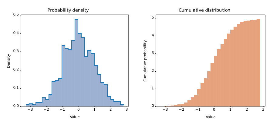
Probability-density and cumulative histograms, with filled and outlined bars.
import numpy as np
import matplotvite as plt

rng = np.random.default_rng(4)
data = rng.normal(loc=0.0, scale=1.0, size=900)
fig, axs = plt.subplots(1, 2, figsize=(9.0, 4.2))
axs[0].hist(data, bins=30, density=True, color="#4c72b0", alpha=0.55,
            label="density")
axs[0].hist(data, bins=30, histtype="step", density=True,
            color="#1f77b4", label="outline")
axs[0].set_title("Probability density")
axs[0].set_xlabel("Value")
axs[0].set_ylabel("Density")
axs[1].hist(data, bins=30, cumulative=True, density=True,
            color="#dd8452", alpha=0.75)
axs[1].set_title("Cumulative distribution")
axs[1].set_xlabel("Value")
axs[1].set_ylabel("Cumulative probability")
fig.savefig("histogram_density.png")
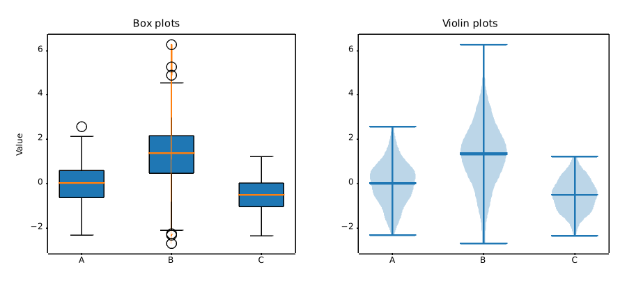
Three sample distributions summarized by box plots and Gaussian-kernel violin plots.
import numpy as np
import matplotvite as plt

rng = np.random.default_rng(11)
groups = [
    rng.normal(0.0, 1.0, 240),
    rng.normal(1.2, 1.4, 240),
    rng.normal(-0.5, 0.7, 240),
]
labels = ["A", "B", "C"]
fig, axs = plt.subplots(1, 2, figsize=(9.0, 4.2))
axs[0].boxplot(groups, patch_artist=True, tick_labels=labels)
axs[0].set_title("Box plots")
axs[0].set_ylabel("Value")
axs[1].violinplot(groups, showmeans=True, showmedians=True)
axs[1].set_xticks([1, 2, 3], labels)
axs[1].set_title("Violin plots")
fig.savefig("box_violin.png")
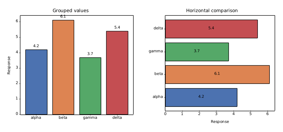
Coloured bar groups with value labels, plus a horizontal comparison.
import numpy as np
import matplotvite as plt

labels = ["alpha", "beta", "gamma", "delta"]
values = np.array([4.2, 6.1, 3.7, 5.4])
colors = ["#4c72b0", "#dd8452", "#55a868", "#c44e52"]
positions = np.arange(len(labels))
fig, axs = plt.subplots(1, 2, figsize=(9.0, 4.2))
bars = axs[0].bar(positions, values, color=colors, edgecolor="black",
                  linewidth=0.6)
axs[0].bar_label(bars, fmt="%.1f", padding=2)
axs[0].set_xticks(positions, labels)
axs[0].set_ylabel("Response")
axs[0].set_title("Grouped values")
hbars = axs[1].barh(positions, values, color=colors, edgecolor="black",
                    linewidth=0.6)
axs[1].bar_label(hbars, fmt="%.1f", label_type="center")
axs[1].set_yticks(positions, labels)
axs[1].set_xlabel("Response")
axs[1].set_title("Horizontal comparison")
fig.savefig("bar_labels.png")
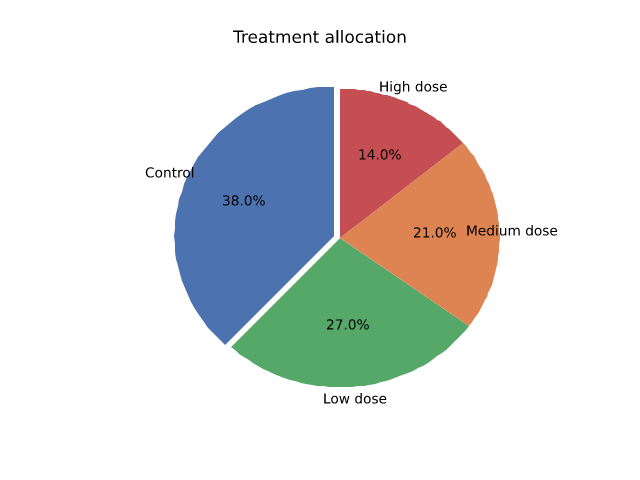
A pie chart with exploded wedges, explicit colours, and percentage labels.
import matplotvite as plt

labels = ["Control", "Low dose", "Medium dose", "High dose"]
sizes = [38, 27, 21, 14]
colors = ["#4c72b0", "#55a868", "#dd8452", "#c44e52"]
plt.figure(figsize=(6.4, 4.8))
plt.pie(sizes, labels=labels, colors=colors, autopct="%1.1f%%",
        explode=(0.04, 0.0, 0.0, 0.0), startangle=90)
plt.title("Treatment allocation")
plt.savefig("pie_chart.png")
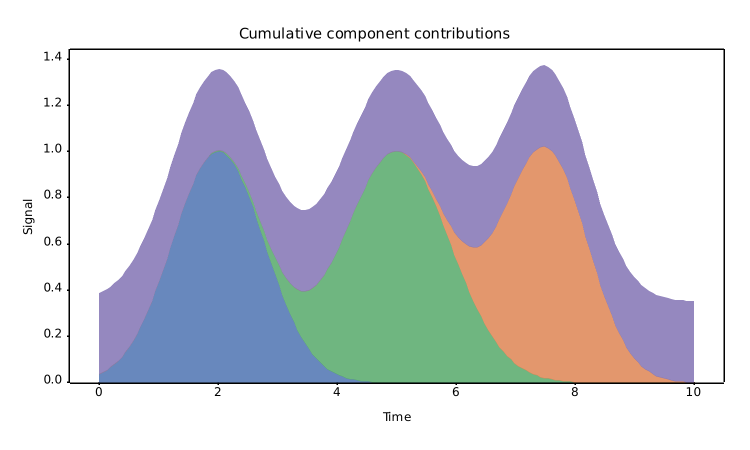
A stackplot showing four components with a symmetric baseline.
import numpy as np
import matplotvite as plt

x = np.linspace(0, 10, 160)
components = [
    np.exp(-((x - 2.0) ** 2) / 1.2),
    np.exp(-((x - 5.0) ** 2) / 1.6),
    np.exp(-((x - 7.5) ** 2) / 1.0),
    0.35 * np.ones_like(x),
]
plt.figure(figsize=(7.5, 4.5))
plt.stackplot(x, *components, labels=["early", "middle", "late", "baseline"],
              colors=["#4c72b0", "#55a868", "#dd8452", "#8172b3"], alpha=0.85)
plt.title("Cumulative component contributions")
plt.xlabel("Time")
plt.ylabel("Signal")
plt.savefig("stackplot.png")
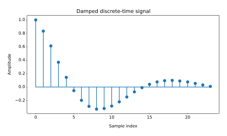
Discrete-time samples rendered as stems with a shared baseline.
import numpy as np
import matplotvite as plt

n = np.arange(24)
y = np.exp(-n / 8.0) * np.cos(n / 3.0)
plt.figure(figsize=(7.5, 4.5))
plt.stem(n, y, linefmt="-", markerfmt="o", basefmt="-")
plt.title("Damped discrete-time signal")
plt.xlabel("Sample index")
plt.ylabel("Amplitude")
plt.savefig("stem_signal.png")
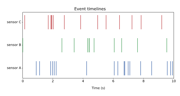
Eventplot rows with distinct colours and offsets, useful for spike and event data.
import numpy as np
import matplotvite as plt

rng = np.random.default_rng(21)
rows = [
    np.sort(rng.uniform(0, 10, 18)),
    np.sort(rng.uniform(0, 10, 11)),
    np.sort(rng.uniform(0, 10, 14)),
]
plt.figure(figsize=(7.5, 4.0))
plt.eventplot(rows, lineoffsets=[1.0, 2.0, 3.0],
              colors=["#4c72b0", "#55a868", "#c44e52"], linelengths=0.6)
plt.yticks([1, 2, 3], ["sensor A", "sensor B", "sensor C"])
plt.xlim(0, 10)
plt.xlabel("Time (s)")
plt.title("Event timelines")
plt.savefig("event_timeline.png")
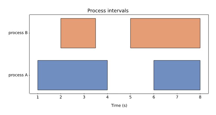
Interval data drawn as broken horizontal bars, including edge colour and alpha.
import matplotvite as plt

plt.figure(figsize=(7.5, 4.0))
plt.broken_barh([(1, 3), (6, 2)], (2, 0.7), facecolors="#4c72b0",
                edgecolor="black", alpha=0.8)
plt.broken_barh([(2, 1.5), (5, 3)], (3, 0.7), facecolors="#dd8452",
                edgecolor="black", alpha=0.8)
plt.yticks([2.35, 3.35], ["process A", "process B"])
plt.xlabel("Time (s)")
plt.title("Process intervals")
plt.savefig("broken_barh.png")
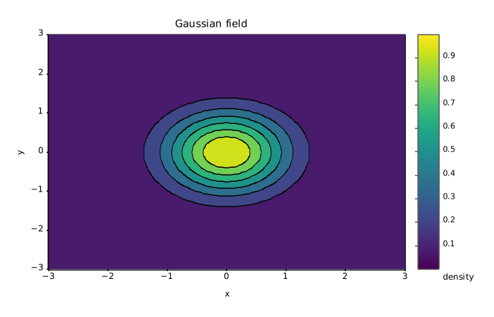
Filled iso-bands of a two-dimensional Gaussian field, with line contours and a colour scale.
import numpy as np
import matplotvite as plt

x = np.linspace(-3, 3, 120)
y = np.linspace(-3, 3, 120)
z = np.exp(-(x[None, :] ** 2 + y[:, None] ** 2))
plt.figure(figsize=(7.0, 4.5))
plt.contourf(x, y, z, levels=8, cmap="viridis")
plt.contour(x, y, z, levels=8, colors="black", linewidths=0.4)
plt.colorbar(label="density")
plt.title("Gaussian field")
plt.xlabel("x")
plt.ylabel("y")
plt.savefig("contours_colorbar.png")
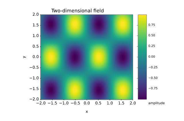
A matrix rendered through imshow with a physical extent and a colourbar.
import numpy as np
import matplotvite as plt

x = np.linspace(-2, 2, 240)
y = np.linspace(-2, 2, 140)
z = np.sin(3 * x[None, :]) * np.cos(2 * y[:, None])
plt.figure(figsize=(6.4, 4.2))
plt.imshow(z, cmap="viridis", extent=(-2, 2, -2, 2), origin="lower")
plt.colorbar(label="amplitude")
plt.title("Two-dimensional field")
plt.xlabel("x")
plt.ylabel("y")
plt.savefig("imshow_heatmap.png")
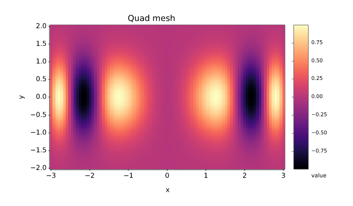
A non-uniform coordinate grid drawn with pcolormesh and a colourbar.
import numpy as np
import matplotvite as plt

x = np.linspace(-3, 3, 90)
y = np.linspace(-2, 2, 70)
z = np.sin(x[None, :] ** 2) * np.exp(-y[:, None] ** 2)
plt.figure(figsize=(7.2, 4.2))
plt.pcolormesh(x, y, z, cmap="magma", shading="auto")
plt.colorbar(label="value")
plt.title("Quad mesh")
plt.xlabel("x")
plt.ylabel("y")
plt.savefig("pcolormesh.png")
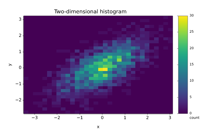
A two-dimensional histogram and hexagonal binning of the same point cloud.
import numpy as np
import matplotvite as plt

rng = np.random.default_rng(5)
x = rng.normal(0, 1, 2400)
y = 0.6 * x + rng.normal(0, 0.7, x.size)
fig, ax = plt.subplots(figsize=(6.8, 4.4))
hist = ax.hist2d(x, y, bins=32, cmap="viridis")
fig.colorbar(hist[3], label="count")
ax.set_title("Two-dimensional histogram")
ax.set_xlabel("x")
ax.set_ylabel("y")
fig.savefig("hist2d_hexbin.png")
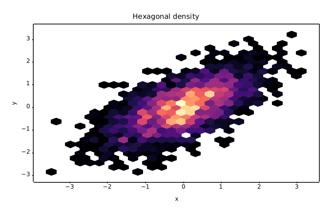
Hexagonal binning of a correlated point cloud with a minimum-count threshold.
import numpy as np
import matplotvite as plt

rng = np.random.default_rng(5)
x = rng.normal(0, 1, 2400)
y = 0.6 * x + rng.normal(0, 0.7, x.size)
fig, ax = plt.subplots(figsize=(6.8, 4.4))
ax.hexbin(x, y, gridsize=26, cmap="magma", mincnt=1)
ax.set_title("Hexagonal density")
ax.set_xlabel("x")
ax.set_ylabel("y")
fig.savefig("hexbin_density.png")
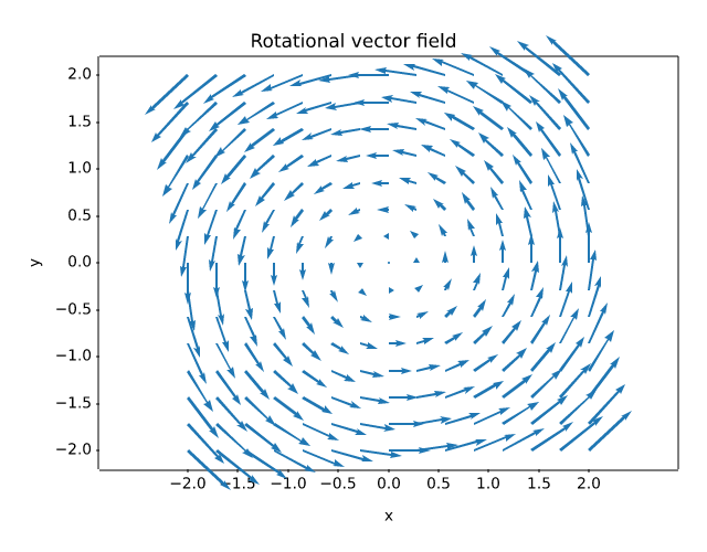
A rotational vector field drawn with quiver on an equal-aspect grid.
import numpy as np
import matplotvite as plt

x = np.linspace(-2, 2, 15)
y = np.linspace(-2, 2, 15)
X, Y = np.meshgrid(x, y)
U, V = -Y, X
plt.figure(figsize=(6.4, 5.0))
plt.quiver(X, Y, U, V, color="#1f77b4", scale=28)
plt.axis("equal")
plt.title("Rotational vector field")
plt.xlabel("x")
plt.ylabel("y")
plt.savefig("quiver_field.png")
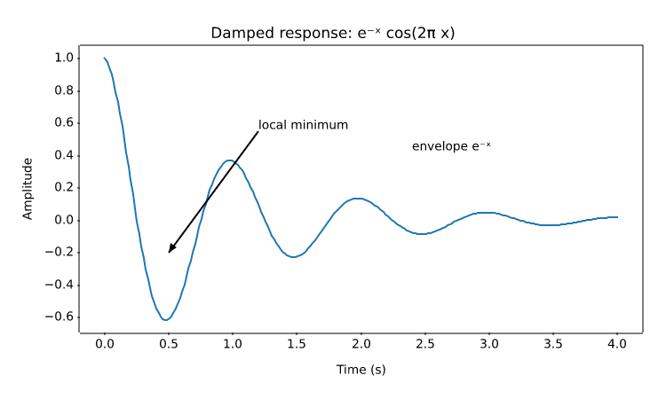
An annotated extremum, axis-fraction text, and the supported mathtext subset.
import numpy as np
import matplotvite as plt

x = np.linspace(0, 4, 240)
y = np.exp(-x) * np.cos(2 * np.pi * x)
plt.figure(figsize=(7.5, 4.5))
plt.plot(x, y, color="#1f77b4", linewidth=1.5)
plt.annotate("local minimum", xy=(0.5, -0.20), xytext=(1.2, 0.55),
             arrowprops=dict(arrowstyle="->", color="#444444"))
plt.text(2.4, 0.42, r"envelope $e^{-x}$", fontsize=10)
plt.title(r"Damped response: $e^{-x} \cos(2\pi x)$")
plt.xlabel("Time (s)")
plt.ylabel("Amplitude")
plt.savefig("annotations_mathtext.png")
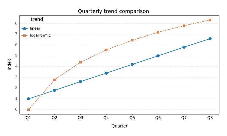
Rotated category labels, styled gridlines, tick parameters, and a two-column legend.
import numpy as np
import matplotvite as plt

x = np.arange(8)
plt.figure(figsize=(7.5, 4.5))
plt.plot(x, 0.8 * x + 1.0, "o-", label="linear", color="#1f77b4")
plt.plot(x, 4.0 * np.log1p(x), "s--", label="logarithmic",
         color="#dd8452")
plt.xticks(x, ["Q1", "Q2", "Q3", "Q4", "Q5", "Q6", "Q7", "Q8"],
           rotation=35, fontsize=9)
plt.tick_params(axis="y", labelsize=9, color="#666666")
plt.grid(True, axis="y", linestyle="--", linewidth=0.7, alpha=0.35)
plt.legend(title="trend", loc="upper left", frameon=False, fontsize=8.5)
plt.title("Quarterly trend comparison")
plt.xlabel("Quarter")
plt.ylabel("Index")
plt.savefig("ticks_grid_legend.png")
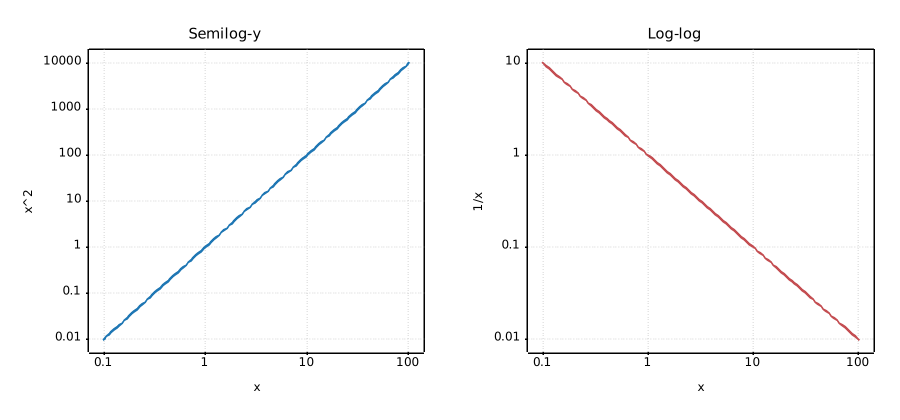
Semilog and log-log axes with explicit scale selection.
import numpy as np
import matplotvite as plt

x = np.logspace(-1, 2, 120)
fig, axs = plt.subplots(1, 2, figsize=(9.0, 4.2))
axs[0].semilogy(x, x ** 2, color="#1f77b4", label="x^2")
axs[0].set_xscale("log")
axs[0].set_title("Semilog-y")
axs[0].set_xlabel("x")
axs[0].set_ylabel("x^2")
axs[1].loglog(x, 1.0 / x, color="#c44e52", label="1/x")
axs[1].set_title("Log-log")
axs[1].set_xlabel("x")
axs[1].set_ylabel("1/x")
for ax in axs:
    ax.grid(True, which="major", linestyle=":", alpha=0.35)
fig.savefig("log_scales.png")
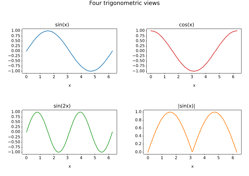
A four-panel figure built with the object-oriented subplots API.
import numpy as np
import matplotvite as plt

x = np.linspace(0, 2 * np.pi, 220)
fig, axs = plt.subplots(2, 2, figsize=(8.5, 6.0))
axs[0, 0].plot(x, np.sin(x), color="#1f77b4")
axs[0, 0].set_title("sin(x)")
axs[0, 1].plot(x, np.cos(x), color="#d62728")
axs[0, 1].set_title("cos(x)")
axs[1, 0].plot(x, np.sin(2 * x), color="#2ca02c")
axs[1, 0].set_title("sin(2x)")
axs[1, 1].plot(x, np.abs(np.sin(x)), color="#ff7f0e")
axs[1, 1].set_title("|sin(x)|")
for ax in axs.flat:
    ax.set_xlabel("x")
fig.suptitle("Four trigonometric views", fontsize=14)
fig.savefig("subplots_grid.png")
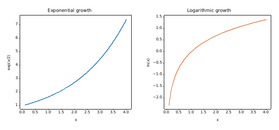
Two comparative panels created with the pyplot subplot() interface.
import numpy as np
import matplotvite as plt

x = np.linspace(0.1, 4.0, 180)
plt.figure(figsize=(9.0, 4.2))
plt.subplot(1, 2, 1)
plt.plot(x, np.exp(x / 2), color="#1f77b4", label="exp(x/2)")
plt.title("Exponential growth")
plt.xlabel("x")
plt.ylabel("exp(x/2)")
plt.subplot(1, 2, 2)
plt.plot(x, np.log(x), color="#dd8452", label="ln(x)")
plt.title("Logarithmic growth")
plt.xlabel("x")
plt.ylabel("ln(x)")
plt.savefig("side_by_side.png")
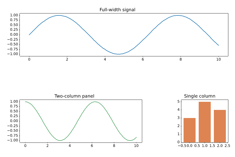
A header panel spanning three columns, with two lower panels of unequal width.
import numpy as np
import matplotvite as plt

fig = plt.figure(figsize=(9.0, 6.0))
gs = fig.add_gridspec(2, 3)
top = fig.add_subplot(gs[0, :])
left = fig.add_subplot(gs[1, 0:2])
right = fig.add_subplot(gs[1, 2])
x = np.linspace(0, 10, 180)
top.plot(x, np.sin(x), color="#1f77b4")
top.set_title("Full-width signal")
left.plot(x, np.cos(x), color="#55a868")
left.set_title("Two-column panel")
right.bar([0, 1, 2], [3, 5, 4], color="#dd8452")
right.set_title("Single column")
fig.savefig("gridspec_layout.png")
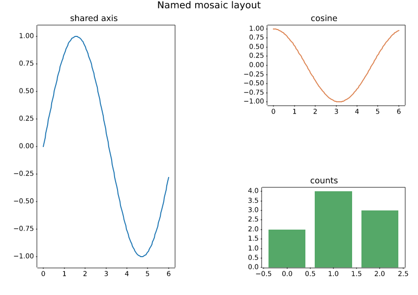
Named panels arranged with subplot_mosaic, including a shared vertical panel.
import numpy as np
import matplotvite as plt

fig, axes = plt.subplot_mosaic(
    [["left", "right"], ["left", "bottom"]], figsize=(8.5, 6.0)
)
x = np.linspace(0, 6, 150)
axes["left"].plot(x, np.sin(x), color="#1f77b4")
axes["left"].set_title("shared axis")
axes["right"].plot(x, np.cos(x), color="#dd8452")
axes["right"].set_title("cosine")
axes["bottom"].bar([0, 1, 2], [2, 4, 3], color="#55a868")
axes["bottom"].set_title("counts")
fig.suptitle("Named mosaic layout", fontsize=14)
fig.savefig("mosaic_layout.png")
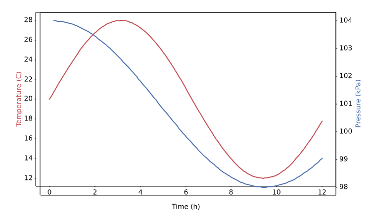
Two measured quantities with independent y scales sharing the same x axis.
import numpy as np
import matplotvite as plt

x = np.linspace(0, 12, 140)
temperature = 20 + 8 * np.sin(x / 2.0)
pressure = 101 + 3 * np.cos(x / 3.0)
fig, ax_left = plt.subplots(figsize=(7.5, 4.5))
ax_left.plot(x, temperature, color="#c44e52", label="temperature")
ax_left.set_xlabel("Time (h)")
ax_left.set_ylabel("Temperature (C)", color="#c44e52")
ax_right = ax_left.twinx()
ax_right.plot(x, pressure, color="#4c72b0", label="pressure")
ax_right.set_ylabel("Pressure (kPa)", color="#4c72b0")
fig.savefig("twin_axes.png")
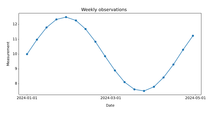
datetime values mapped to matplotlib date numbers with calendar-aligned ticks.
from datetime import datetime, timedelta

import numpy as np
import matplotvite as plt

start = datetime(2024, 1, 1)
dates = [start + timedelta(days=7 * i) for i in range(18)]
values = 10 + 2.5 * np.sin(np.arange(len(dates)) / 2.5)
plt.figure(figsize=(8.0, 4.4))
plt.plot(dates, values, "o-", color="#1f77b4", markersize=4)
plt.xticks([datetime(2024, 1, 1), datetime(2024, 3, 1),
            datetime(2024, 5, 1)])
plt.title("Weekly observations")
plt.xlabel("Date")
plt.ylabel("Measurement")
plt.savefig("datetime_axis.png")
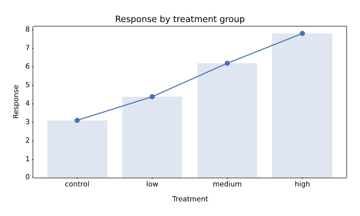
String categories converted to stable numeric positions and rendered as tick labels.
import numpy as np
import matplotvite as plt

categories = ["control", "low", "medium", "high"]
values = np.array([3.1, 4.4, 6.2, 7.8])
plt.figure(figsize=(7.0, 4.2))
plt.plot(categories, values, "o-", color="#4c72b0", markersize=6)
plt.bar(categories, values, color="#4c72b0", alpha=0.18)
plt.title("Response by treatment group")
plt.xlabel("Treatment")
plt.ylabel("Response")
plt.savefig("categorical_axis.png")
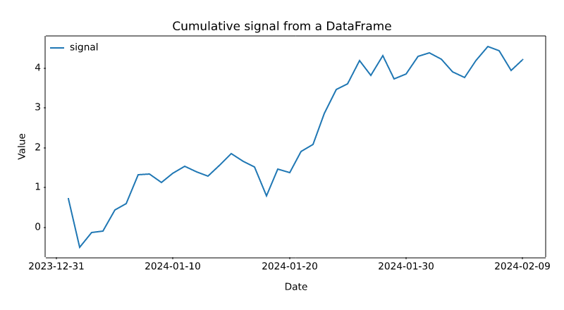
Plotting named columns directly from a pandas DataFrame, with its date index.
import numpy as np
import pandas as pd
import matplotvite as plt

rng = np.random.default_rng(13)
dates = pd.date_range("2024-01-01", periods=40, freq="D")
frame = pd.DataFrame(
    {"signal": np.cumsum(rng.normal(0, 0.4, dates.size))},
    index=dates,
)
plt.figure(figsize=(8.0, 4.4))
plt.plot("signal", data=frame, label="signal", color="#1f77b4")
plt.title("Cumulative signal from a DataFrame")
plt.xlabel("Date")
plt.ylabel("Value")
plt.legend(frameon=False, loc="upper left")
plt.savefig("pandas_frame.png")
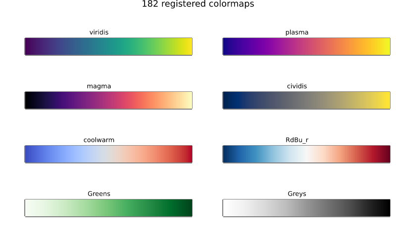
A sample of the registered colormaps, all available without a matplotlib dependency.
import numpy as np
import matplotvite as plt

names = ["viridis", "plasma", "magma", "cividis",
         "coolwarm", "RdBu_r", "Greens", "Greys"]
gradient = np.linspace(0, 1, 256)[None, :]
fig, axs = plt.subplots(4, 2, figsize=(8.0, 4.8))
for ax, name in zip(axs.flat, names):
    ax.imshow(gradient, cmap=name, aspect="auto")
    ax.set_title(name, fontsize=9)
    ax.set_xticks([])
    ax.set_yticks([])
fig.suptitle(f"{len(plt.colormaps())} registered colormaps", fontsize=13)
fig.savefig("colormap_reference.png")
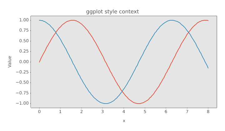
A scoped style preset that changes figure colours and lines without leaking state.
import numpy as np
import matplotvite as plt

x = np.linspace(0, 8, 160)
with plt.style.context("ggplot"):
    fig, ax = plt.subplots(figsize=(7.2, 4.2))
    ax.plot(x, np.sin(x), label="sin(x)", linewidth=1.6)
    ax.plot(x, np.cos(x), label="cos(x)", linewidth=1.6)
    ax.set_title("ggplot style context")
    ax.set_xlabel("x")
    ax.set_ylabel("Value")
    fig.savefig("style_context.png")
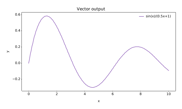
Resolution-independent SVG output with text and vector paths preserved.
import numpy as np
import matplotvite as plt

x = np.linspace(0, 10, 250)
y = np.sin(x) / (0.5 * x + 1.0)
plt.figure(figsize=(7.5, 4.5))
plt.plot(x, y, label="sin(x)/(0.5x+1)", color="#9467bd")
plt.title("Vector output")
plt.xlabel("x")
plt.ylabel("y")
plt.legend(frameon=False, loc="upper right")
plt.savefig("svg_export.svg")
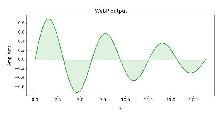
Lossless WebP encoding from the same rendering path used for PNG.
import numpy as np
import matplotvite as plt

x = np.linspace(0, 6 * np.pi, 400)
plt.figure(figsize=(7.5, 4.0))
plt.plot(x, np.sin(x) * np.exp(-x / 14), color="#2ca02c")
plt.fill_between(x, np.sin(x) * np.exp(-x / 14), 0,
                 color="#2ca02c", alpha=0.15)
plt.title("WebP output")
plt.xlabel("x")
plt.ylabel("Amplitude")
plt.savefig("webp_export.webp")